pertpy.tools.Tasccoda
- class pertpy.tools.Tasccoda(*args, **kwargs)[source]
Statistical model for tree-aggregated differential composition analysis (tascCODA, Ostner et al., 2021).
The hierarchical formulation of the model for one sample is:
\[\begin{split}\begin{align*} Y_i &\sim \textrm{DirMult}(\bar{Y}_i, \textbf{a}(\textbf{x})_i)\\ \log(\textbf{a}(X))_i &= \alpha + X_{i, \cdot} \beta\\ \alpha_j &\sim \mathcal{N}(0, 10) & \forall j\in[p]\\ \beta &= \hat{\beta} A^T \\ \hat{\beta}_{l, k} &= 0 & \forall k \in \hat{v}, l \in [d]\\ \hat{\beta}_{l, k} &= \theta \tilde{\beta}_{1, l, k} + (1- \theta) \tilde{\beta}_{0, l, k} \quad & \forall k\in\{[v] \smallsetminus \hat{v}\}, l \in [d]\\ \tilde{\beta}_{m, l, k} &= \sigma_{m, l, k} * b_{m, l, k} \quad & \forall k\in\{[v] \smallsetminus \hat{v}\}, m \in \{0, 1\}, l \in [d]\\ \sigma_{m, l, k} &\sim \textrm{Exp}(\lambda_{m, l, k}^2/2) \quad & \forall k\in\{[v] \smallsetminus \hat{v}\}, l \in \{0, 1\}, l \in [d]\\ b_{m, l, k} &\sim N(0,1) \quad & \forall k\in\{[v] \smallsetminus \hat{v}\}, l \in \{0, 1\}, l \in [d]\\ \theta &\sim \textrm{Beta}(1, \frac{1}{|\{[v] \smallsetminus \hat{v}\}|}) \end{align*}\end{split}\]with Y being the cell counts, X the covariates, and v the set of nodes of the underlying tree structure.
For further information, see tascCODA: Bayesian Tree-Aggregated Analysis of Compositional Amplicon and Single-Cell Data (Ostner et al., 2021)
Methods table
|
Decides which effects of the scCODA model are credible based on an adjustable inclusion probability threshold. |
|
Get effect dataframe as printed in the extended summary |
|
Get intercept dataframe as printed in the extended summary |
|
Get node effect dataframe as printed in the extended summary of a tascCODA model |
|
Prepare a MuData object for subsequent processing. |
|
Creates arviz object from model results for MCMC diagnosis |
|
Implements tascCODA model in numpyro |
|
Handles data preprocessing, covariate matrix creation, reference selection, and zero count replacement for tascCODA. |
|
Run standard Hamiltonian Monte Carlo sampling (Neal, 2011) to infer optimal model parameters. |
|
Run No-U-turn sampling (Hoffman and Gelman, 2014), an efficient version of Hamiltonian Monte Carlo sampling to infer optimal model parameters. |
|
Direct posterior probability approach to calculate credible effects while keeping the expected FDR at a certain level |
|
Sets initial MCMC state values for tascCODA model |
|
Printing method for the summary. |
|
Generates summary dataframes for intercepts, effects and node-level effect (if using tree aggregation). |
|
Grouped boxplot visualization. |
|
Plot a tree with colored circles on the nodes indicating significant effects with bar plots which indicate leave-level significant effects. |
|
Plot a tree using input ete3 tree object. |
|
Barplot visualization for effects. |
|
Plot a UMAP visualization colored by effect strength. |
|
Plots total variance of relative abundance versus minimum relative abundance of all cell types for determination of a reference cell type. |
|
Plots a stacked barplot for all levels of a covariate or all samples (if feature_name=="samples"). |
Methods
credible_effects
- Tasccoda.credible_effects(data, modality_key='coda', est_fdr=None)[source]
- Decides which effects of the scCODA model are credible based on an adjustable inclusion probability threshold.
Note: Parameter est_fdr has no effect for spike-and-slab LASSO selection method
- Parameters:
- Returns:
Credible effect decision series which includes boolean values indicate whether effects are credible under inc_prob_threshold.
- Return type:
pd.Series
Examples
>>> import pertpy as pt
>>> adata = pt.dt.tasccoda_example()
>>> tasccoda = pt.tl.Tasccoda()
>>> mdata = tasccoda.load(
>>>     adata, type="sample_level",
>>>     levels_agg=["Major_l1", "Major_l2", "Major_l3", "Major_l4", "Cluster"],
>>>     key_added="lineage", add_level_name=True
>>> )
>>> mdata = tasccoda.prepare(
>>>     mdata, formula="Health", reference_cell_type="automatic", tree_key="lineage", pen_args={"phi": 0}
>>> )
>>> tasccoda.run_nuts(mdata, num_samples=1000, num_warmup=100, rng_key=42)
>>> tasccoda.credible_effects(mdata)
get_effect_df
- Tasccoda.get_effect_df(data, modality_key='coda')
Get effect dataframe as printed in the extended summary
- Parameters:
- Returns:
Effect data frame.
- Return type:
pd.DataFrame
Examples
>>> import pertpy as pt
>>> haber_cells = pt.dt.haber_2017_regions()
>>> sccoda = pt.tl.Sccoda()
>>> mdata = sccoda.load(haber_cells, type="cell_level", generate_sample_level=True, cell_type_identifier="cell_label",                 sample_identifier="batch", covariate_obs=["condition"])
>>> mdata = sccoda.prepare(mdata, formula="condition", reference_cell_type="Endocrine")
>>> sccoda.run_nuts(mdata, num_warmup=100, num_samples=1000, rng_key=42)
>>> effects = sccoda.get_effect_df(mdata)
get_intercept_df
- Tasccoda.get_intercept_df(data, modality_key='coda')
Get intercept dataframe as printed in the extended summary
- Parameters:
- Returns:
Intercept data frame.
- Return type:
pd.DataFrame
Examples
>>> import pertpy as pt
>>> haber_cells = pt.dt.haber_2017_regions()
>>> sccoda = pt.tl.Sccoda()
>>> mdata = sccoda.load(haber_cells, type="cell_level", generate_sample_level=True, cell_type_identifier="cell_label",                 sample_identifier="batch", covariate_obs=["condition"])
>>> mdata = sccoda.prepare(mdata, formula="condition", reference_cell_type="Endocrine")
>>> sccoda.run_nuts(mdata, num_warmup=100, num_samples=1000, rng_key=42)
>>> intercepts = sccoda.get_intercept_df(mdata)
get_node_df
- Tasccoda.get_node_df(data, modality_key='coda')
Get node effect dataframe as printed in the extended summary of a tascCODA model
- Parameters:
- Returns:
Node effect data frame.
- Return type:
pd.DataFrame
Examples
>>> import pertpy as pt
>>> adata = pt.dt.tasccoda_example()
>>> tasccoda = pt.tl.Tasccoda()
>>> mdata = tasccoda.load(
>>>     adata, type="sample_level",
>>>     levels_agg=["Major_l1", "Major_l2", "Major_l3", "Major_l4", "Cluster"],
>>>     key_added="lineage", add_level_name=True
>>> )
>>> mdata = tasccoda.prepare(
>>>     mdata, formula="Health", reference_cell_type="automatic", tree_key="lineage", pen_args={"phi": 0}
>>> )
>>> tasccoda.run_nuts(mdata, num_samples=1000, num_warmup=100, rng_key=42)
>>> node_effects = tasccoda.get_node_df(mdata)
load
- Tasccoda.load(adata, type, cell_type_identifier=None, sample_identifier=None, covariate_uns=None, covariate_obs=None, covariate_df=None, dendrogram_key=None, levels_orig=None, levels_agg=None, add_level_name=True, key_added='tree', modality_key_1='rna', modality_key_2='coda')[source]
Prepare a MuData object for subsequent processing. If type is “cell_level”, then create a compositional analysis dataset from the input adata. If type is “sample_level”, generate ete tree for tascCODA models from dendrogram information or cell-level observations.
When using
type="cell_level",adataneeds to have a column inadata.obsthat contains the cell type assignment. Further, it must contain one column or a set of columns (e.g. subject id, treatment, disease status) that uniquely identify each (statistical) sample. Further covariates (e.g. subject age) can either be specified via addidional column names inadata.obs, a key inadata.uns, or as a separate DataFrame.- Parameters:
adata (
AnnData) – AnnData object.type (
Literal['cell_level','sample_level']) – Specify the input adata type, which could be either a cell-level AnnData or an aggregated sample-level AnnData.cell_type_identifier (
str) – If type is “cell_level”, specify column name in adata.obs that specifies the cell types. Defaults to None.sample_identifier (
str) – If type is “cell_level”, specify column name in adata.obs that specifies the sample. Defaults to None.covariate_uns (
str|None) – If type is “cell_level”, specify key for adata.uns, where covariate values are stored. Defaults to None.covariate_obs (
list[str] |None) – If type is “cell_level”, specify list of keys for adata.obs, where covariate values are stored. Defaults to None.covariate_df (
DataFrame|None) – If type is “cell_level”, specify dataFrame with covariates. Defaults to None.dendrogram_key (
str) – Key to the scanpy.tl.dendrogram result in .uns of original cell level anndata object. Defaults to None.levels_orig (
list[str]) – List that indicates which columns in .obs of the original data correspond to tree levels. The list must begin with the root level, and end with the leaf level. Defaults to None.levels_agg (
list[str]) – List that indicates which columns in .var of the aggregated data correspond to tree levels. The list must begin with the root level, and end with the leaf level. Defaults to None.add_level_name (
bool) – If True, internal nodes in the tree will be named as “{level_name}_{node_name}” instead of just {level_name}. Defaults to False.key_added (
str) – If not specified, the tree is stored in .uns[‘tree’]. If data is AnnData, save tree in data. If data is MuData, save tree in data[modality_2]. Defaults to “tree”.modality_key_1 (
str) – Key to the cell-level AnnData in the MuData object. Defaults to “rna”.modality_key_2 (
str) – Key to the aggregated sample-level AnnData object in the MuData object. Defaults to “coda”.
- Returns:
MuData object with cell-level AnnData (mudata[modality_key_1]) and aggregated sample-level AnnData (mudata[modality_key_2]).
- Return type:
MuData
Examples
>>> import pertpy as pt
>>> adata = pt.dt.tasccoda_example()
>>> tasccoda = pt.tl.Tasccoda()
>>> mdata = tasccoda.load(
>>>     adata, type="sample_level",
>>>     levels_agg=["Major_l1", "Major_l2", "Major_l3", "Major_l4", "Cluster"],
>>>     key_added="lineage", add_level_name=True
>>> )
make_arviz
- Tasccoda.make_arviz(data, modality_key='coda', rng_key=None, num_prior_samples=500, use_posterior_predictive=True)[source]
Creates arviz object from model results for MCMC diagnosis
- Parameters:
data (
AnnData|MuData) – AnnData object or MuData object.modality_key (
str) – If data is a MuData object, specify which modality to use. Defaults to “coda”.rng_key – The rng state used for the prior simulation. If None, a random state will be selected. Defaults to None.
num_prior_samples (
int) – Number of prior samples calculated. Defaults to 500.use_posterior_predictive (
bool) – If True, the posterior predictive will be calculated. Defaults to True.
- Returns:
arviz_data
- Return type:
arviz.InferenceData
Examples
>>> import pertpy as pt
>>> adata = pt.dt.tasccoda_example()
>>> tasccoda = pt.tl.Tasccoda()
>>> mdata = tasccoda.load(
>>>     adata, type="sample_level",
>>>     levels_agg=["Major_l1", "Major_l2", "Major_l3", "Major_l4", "Cluster"],
>>>     key_added="lineage", add_level_name=True
>>> )
>>> mdata = tasccoda.prepare(
>>>     mdata, formula="Health", reference_cell_type="automatic", tree_key="lineage", pen_args={"phi": 0}
>>> )
>>> tasccoda.run_nuts(mdata, num_samples=1000, num_warmup=100, rng_key=42)
>>> arviz_data = tasccoda.make_arviz(mdata)
model
plot_boxplots
- Tasccoda.plot_boxplots(data, feature_name, modality_key='coda', y_scale='relative', plot_facets=False, add_dots=False, cell_types=None, args_boxplot=None, args_swarmplot=None, palette='Blues', show_legend=True, level_order=None, figsize=None, dpi=100, return_fig=None, ax=None, show=None, save=None)
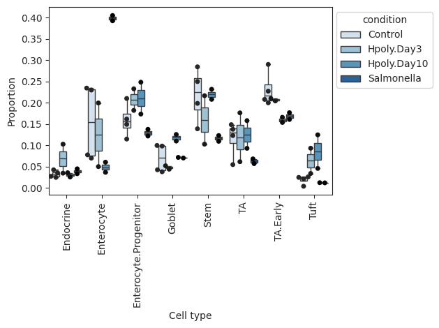
Grouped boxplot visualization.
The cell counts for each cell type are shown as a group of boxplots with intra–group separation by a covariate from data.obs.
- Parameters:
data (
AnnData|MuData) – AnnData object or MuData objectfeature_name (
str) – The name of the feature in data.obs to plotmodality_key (
str) – If data is a MuData object, specify which modality to use. Defaults to “coda”.y_scale (
Literal['relative','log','log10','count']) – Transformation to of cell counts. Options: “relative” - Relative abundance, “log” - log(count), “log10” - log10(count), “count” - absolute abundance (cell counts). Defaults to “relative”.plot_facets (
bool) – If False, plot cell types on the x-axis. If True, plot as facets. Defaults to False.add_dots (
bool) – If True, overlay a scatterplot with one dot for each data point. Defaults to False.cell_types (
list|None) – Subset of cell types that should be plotted. Defaults to None.args_boxplot (
dict|None) – Arguments passed to sns.boxplot. Defaults to {}.args_swarmplot (
dict|None) – Arguments passed to sns.swarmplot. Defaults to {}.figsize (
tuple[float,float] |None) – Figure size. Defaults to None.palette (
str|None) – The seaborn color map for the barplot. Defaults to “Blues”.show_legend (
bool|None) – If True, adds a legend. Defaults to True.level_order (
list[str]) – Custom ordering of bars on the x-axis. Defaults to None.
- Return type:
- Returns:
Depending on plot_facets, returns a
Axes(plot_facets = False) orFacetGrid(plot_facets = True) object
Examples
>>> import pertpy as pt
>>> haber_cells = pt.dt.haber_2017_regions()
>>> sccoda = pt.tl.Sccoda()
>>> mdata = sccoda.load(haber_cells, type="cell_level", generate_sample_level=True, cell_type_identifier="cell_label",                 sample_identifier="batch", covariate_obs=["condition"])
>>> sccoda.plot_boxplots(mdata, feature_name="condition", add_dots=True)
- Preview:
plot_draw_effects
- Tasccoda.plot_draw_effects(data, covariate, modality_key='coda', tree='tree', show_legend=None, show_leaf_effects=False, tight_text=False, show_scale=False, units='px', figsize=(None, None), dpi=100, show=True, save=None)
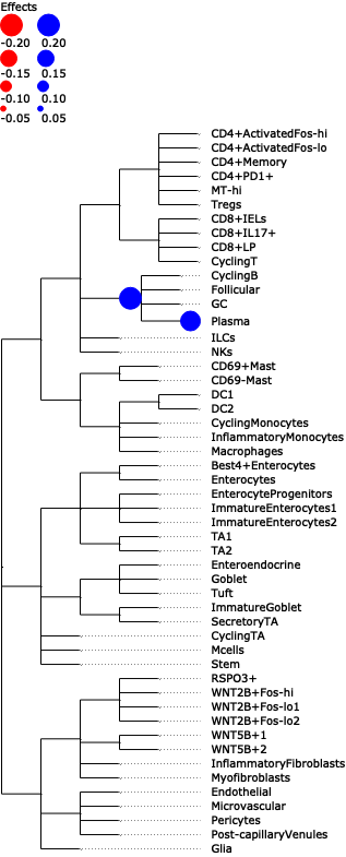
Plot a tree with colored circles on the nodes indicating significant effects with bar plots which indicate leave-level significant effects.
- Parameters:
data (
AnnData|MuData) – AnnData object or MuData object.covariate (
str) – The covariate, whose effects should be plotted.modality_key (
str) – If data is a MuData object, specify which modality to use. Defaults to “coda”.tree (
str) – A ete3 tree object or a str to indicate the tree stored in .uns. Defaults to “tree”.show_legend (
bool|None) – If show legend of nodes significant effects or not. Defaults to False if show_leaf_effects is True.show_leaf_effects (
bool|None) – If True, plot bar plots which indicate leave-level significant effects. Defaults to False.tight_text (
bool|None) – When False, boundaries of the text are approximated according to general font metrics, producing slightly worse aligned text faces but improving the performance of tree visualization in scenes with a lot of text faces. Defaults to False.show_scale (
bool|None) – Include the scale legend in the tree image or not. Defaults to False.show (
bool|None) – If True, plot the tree inline. If false, return tree and tree_style objects. Defaults to True.file_name – Path to the output image file. valid extensions are .SVG, .PDF, .PNG. Output image can be saved whether show is True or not. Defaults to None.
units (
Optional[Literal['px','mm','in']]) – Unit of image sizes. “px”: pixels, “mm”: millimeters, “in”: inches. Defaults to “px”.figsize (
tuple[float,float] |None) – Figure size. Defaults to None.
- Return type:
TreeNode|None- Returns:
Depending on show, returns
ete3.TreeNodeandete3.TreeStyle(show = False) or plot the tree inline (show = False)
Examples
>>> import pertpy as pt
>>> adata = pt.dt.tasccoda_example()
>>> tasccoda = pt.tl.Tasccoda()
>>> mdata = tasccoda.load(
>>>     adata, type="sample_level",
>>>     levels_agg=["Major_l1", "Major_l2", "Major_l3", "Major_l4", "Cluster"],
>>>     key_added="lineage", add_level_name=True
>>> )
>>> mdata = tasccoda.prepare(
>>>     mdata, formula="Health", reference_cell_type="automatic", tree_key="lineage", pen_args={"phi": 0}
>>> )
>>> tasccoda.run_nuts(mdata, num_samples=1000, num_warmup=100, rng_key=42)
>>> tasccoda.plot_draw_effects(mdata, covariate="Health[T.Inflamed]", tree="lineage")
- Preview:
plot_draw_tree
- Tasccoda.plot_draw_tree(data, modality_key='coda', tree='tree', tight_text=False, show_scale=False, units='px', figsize=(None, None), dpi=100, show=True, save=None)
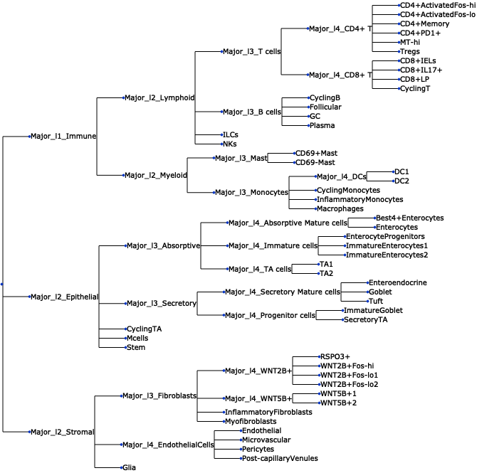
Plot a tree using input ete3 tree object.
- Parameters:
data (
AnnData|MuData) – AnnData object or MuData object.modality_key (
str) – If data is a MuData object, specify which modality to use. Defaults to “coda”.tree (
str) – A ete3 tree object or a str to indicate the tree stored in .uns. Defaults to “tree”.tight_text (
bool|None) – When False, boundaries of the text are approximated according to general font metrics, producing slightly worse aligned text faces but improving the performance of tree visualization in scenes with a lot of text faces. Default to False.show_scale (
bool|None) – Include the scale legend in the tree image or not. Defaults to False.show (
bool|None) – If True, plot the tree inline. If false, return tree and tree_style objects. Defaults to True.file_name – Path to the output image file. Valid extensions are .SVG, .PDF, .PNG. Output image can be saved whether show is True or not. Defaults to None.
units (
Optional[Literal['px','mm','in']]) – Unit of image sizes. “px”: pixels, “mm”: millimeters, “in”: inches. Defaults to “px”.figsize (
tuple[float,float] |None) – Figure size. Defaults to None.
- Return type:
TreeNode|None- Returns:
Depending on show, returns
ete3.TreeNodeandete3.TreeStyle(show = False) or plot the tree inline (show = False)
Examples
>>> import pertpy as pt
>>> adata = pt.dt.tasccoda_example()
>>> tasccoda = pt.tl.Tasccoda()
>>> mdata = tasccoda.load(
>>>     adata, type="sample_level",
>>>     levels_agg=["Major_l1", "Major_l2", "Major_l3", "Major_l4", "Cluster"],
>>>     key_added="lineage", add_level_name=True
>>> )
>>> mdata = tasccoda.prepare(
>>>     mdata, formula="Health", reference_cell_type="automatic", tree_key="lineage", pen_args={"phi": 0}
>>> )
>>> tasccoda.run_nuts(mdata, num_samples=1000, num_warmup=100, rng_key=42)
>>> tasccoda.plot_draw_tree(mdata, tree="lineage")
- Preview:
plot_effects_barplot
- Tasccoda.plot_effects_barplot(data, modality_key='coda', covariates=None, parameter='log2-fold change', plot_facets=True, plot_zero_covariate=True, plot_zero_cell_type=False, palette=<matplotlib.colors.ListedColormap object>, level_order=None, args_barplot=None, figsize=None, dpi=100, return_fig=None, ax=None, show=None, save=None)
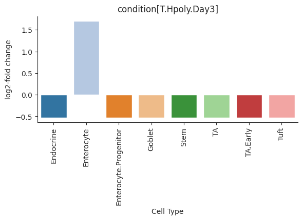
Barplot visualization for effects.
The effect results for each covariate are shown as a group of barplots, with intra–group separation by cell types. The covariates groups can either be ordered along the x-axis of a single plot (plot_facets=False) or as plot facets (plot_facets=True).
- Parameters:
data (
AnnData|MuData) – AnnData object or MuData object.modality_key (
str) – If data is a MuData object, specify which modality to use. Defaults to “coda”.covariates (
str|list|None) – The name of the covariates in data.obs to plot. Defaults to None.parameter (
Literal['log2-fold change','Final Parameter','Expected Sample']) – The parameter in effect summary to plot. Defaults to “log2-fold change”.plot_facets (
bool) – If False, plot cell types on the x-axis. If True, plot as facets. Defaults to True.plot_zero_covariate (
bool) – If True, plot covariate that have all zero effects. If False, do not plot. Defaults to True.plot_zero_cell_type (
bool) – If True, plot cell type that have zero effect. If False, do not plot. Defaults to False.figsize (
tuple[float,float] |None) – Figure size. Defaults to None.palette (
str|ListedColormap|None) – The seaborn color map for the barplot. Defaults to cm.tab20.level_order (
list[str]) – Custom ordering of bars on the x-axis. Defaults to None.args_barplot (
dict|None) – Arguments passed to sns.barplot. Defaults to None.
- Return type:
- Returns:
Depending on plot_facets, returns a
Axes(plot_facets = False) orFacetGrid(plot_facets = True) object
Examples
>>> import pertpy as pt
>>> haber_cells = pt.dt.haber_2017_regions()
>>> sccoda = pt.tl.Sccoda()
>>> mdata = sccoda.load(haber_cells, type="cell_level", generate_sample_level=True, cell_type_identifier="cell_label",                 sample_identifier="batch", covariate_obs=["condition"])
>>> mdata = sccoda.prepare(mdata, formula="condition", reference_cell_type="Endocrine")
>>> sccoda.run_nuts(mdata, num_warmup=100, num_samples=1000, rng_key=42)
>>> sccoda.plot_effects_barplot(mdata)
- Preview:
plot_effects_umap
- Tasccoda.plot_effects_umap(mdata, effect_name, cluster_key, modality_key_1='rna', modality_key_2='coda', color_map=None, palette=None, return_fig=None, ax=None, show=None, save=None, **kwargs)
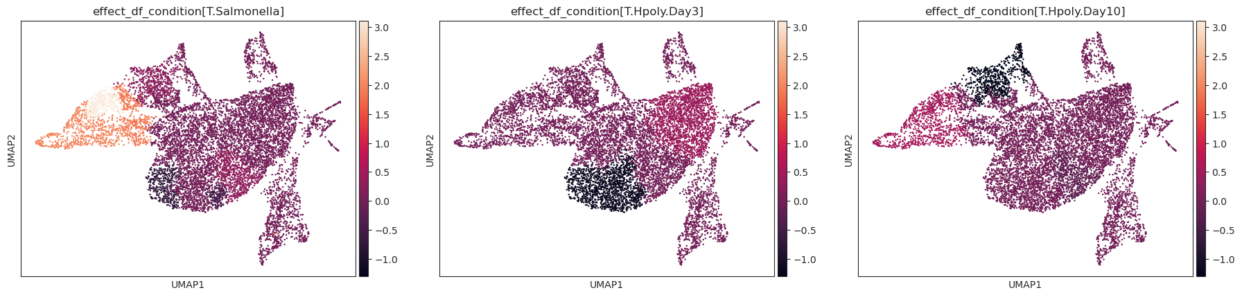
Plot a UMAP visualization colored by effect strength.
Effect results in .varm of aggregated sample-level AnnData (default is data[‘coda’]) are assigned to cell-level AnnData (default is data[‘rna’]) depending on the cluster they were assigned to.
- Parameters:
mudata – MuData object.
effect_name (
str|list|None) – The name of the effect results in .varm of aggregated sample-level AnnData to plotcluster_key (
str) – The cluster information in .obs of cell-level AnnData (default is data[‘rna’]). To assign cell types’ effects to original cells.modality_key_1 (
str) – Key to the cell-level AnnData in the MuData object. Defaults to “rna”.modality_key_2 (
str) – Key to the aggregated sample-level AnnData object in the MuData object. Defaults to “coda”.show (
bool) – Whether to display the figure or return axis. Defaults to None.ax (
Axes) – A matplotlib axes object. Only works if plotting a single component. Defaults to None.**kwargs – All other keyword arguments are passed to scanpy.plot.umap()
- Return type:
- Returns:
If show==False a
Axesor a list of it.
Examples
>>> import pertpy as pt
>>> import scanpy as sc
>>> import schist
>>> adata = pt.dt.haber_2017_regions()
>>> sc.pp.neighbors(adata)
>>> schist.inference.nested_model(adata, n_init=100, random_seed=5678)
>>> tasccoda_model = pt.tl.Tasccoda()
>>> tasccoda_data = tasccoda_model.load(adata, type="cell_level",
>>>                 cell_type_identifier="nsbm_level_1",
>>>                 sample_identifier="batch", covariate_obs=["condition"],
>>>                 levels_orig=["nsbm_level_4", "nsbm_level_3", "nsbm_level_2", "nsbm_level_1"],
>>>                 add_level_name=True)
>>> tasccoda_model.prepare(
>>>     tasccoda_data,
>>>     modality_key="coda",
>>>     reference_cell_type="18",
>>>     formula="condition",
>>>     pen_args={"phi": 0, "lambda_1": 3.5},
>>>     tree_key="tree"
>>> )
>>> tasccoda_model.run_nuts(
...     tasccoda_data, modality_key="coda", rng_key=1234, num_samples=10000, num_warmup=1000
... )
>>> tasccoda_model.run_nuts(
...     tasccoda_data, modality_key="coda", rng_key=1234, num_samples=10000, num_warmup=1000
... )
>>> sc.tl.umap(tasccoda_data["rna"])
>>> tasccoda_model.plot_effects_umap(tasccoda_data,
>>>                         effect_name=["effect_df_condition[T.Salmonella]",
>>>                                      "effect_df_condition[T.Hpoly.Day3]",
>>>                                      "effect_df_condition[T.Hpoly.Day10]"],
>>>                                       cluster_key="nsbm_level_1",
>>>                         )
- Preview:
plot_rel_abundance_dispersion_plot
- Tasccoda.plot_rel_abundance_dispersion_plot(data, modality_key='coda', abundant_threshold=0.9, default_color='Grey', abundant_color='Red', label_cell_types=True, figsize=None, dpi=100, return_fig=None, ax=None, show=None, save=None)
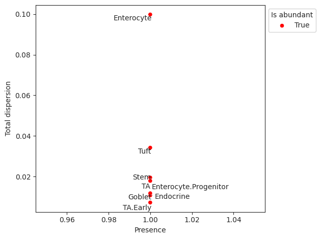
Plots total variance of relative abundance versus minimum relative abundance of all cell types for determination of a reference cell type.
If the count of the cell type is larger than 0 in more than abundant_threshold percent of all samples, the cell type will be marked in a different color.
- Parameters:
data (
AnnData|MuData) – AnnData or MuData object.modality_key (
str) – If data is a MuData object, specify which modality to use. Defaults to “coda”. Defaults to “coda”.abundant_threshold (
float|None) – Presence threshold for abundant cell types. Defaults to 0.9.default_color (
str|None) – Bar color for all non-minimal cell types. Defaults to “Grey”.abundant_color (
str|None) – Bar color for cell types with abundant percentage larger than abundant_threshold. Defaults to “Red”.label_cell_types (
bool) – Label dots with cell type names. Defaults to True.figsize (
tuple[float,float] |None) – Figure size. Defaults to None.ax (
Axes|None) – A matplotlib axes object. Only works if plotting a single component. Defaults to None.
- Return type:
- Returns:
A
Axesobject
Examples
>>> import pertpy as pt
>>> haber_cells = pt.dt.haber_2017_regions()
>>> sccoda = pt.tl.Sccoda()
>>> mdata = sccoda.load(haber_cells, type="cell_level", generate_sample_level=True, cell_type_identifier="cell_label",                 sample_identifier="batch", covariate_obs=["condition"])
>>> mdata = sccoda.prepare(mdata, formula="condition", reference_cell_type="Endocrine")
>>> sccoda.run_nuts(mdata, num_warmup=100, num_samples=1000, rng_key=42)
>>> sccoda.plot_rel_abundance_dispersion_plot(mdata)
- Preview:
plot_stacked_barplot
- Tasccoda.plot_stacked_barplot(data, feature_name, modality_key='coda', palette=<matplotlib.colors.ListedColormap object>, show_legend=True, level_order=None, figsize=None, dpi=100, return_fig=None, ax=None, show=None, save=None, **kwargs)
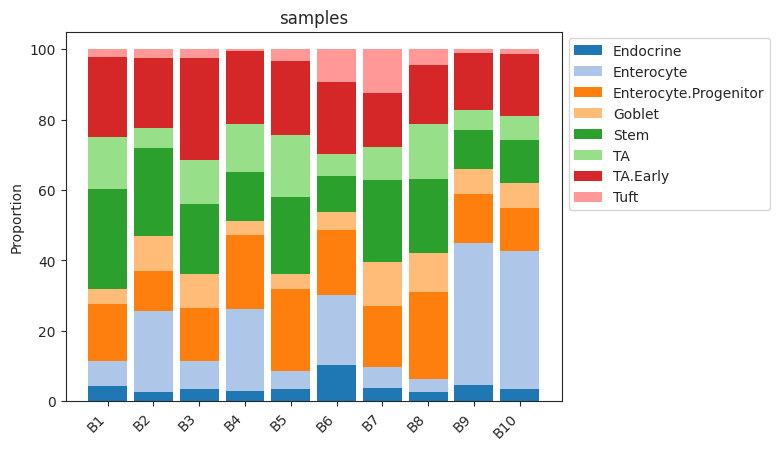
Plots a stacked barplot for all levels of a covariate or all samples (if feature_name==”samples”).
- Parameters:
data (
AnnData|MuData) – AnnData object or MuData object.feature_name (
str) – The name of the covariate to plot. If feature_name==”samples”, one bar for every sample will be plottedmodality_key (
str) – If data is a MuData object, specify which modality to use. Defaults to “coda”.figsize (
tuple[float,float] |None) – Figure size. Defaults to None.palette (
ListedColormap|None) – The matplotlib color map for the barplot. Defaults to cm.tab20.show_legend (
bool|None) – If True, adds a legend. Defaults to True.level_order (
list[str]) – Custom ordering of bars on the x-axis. Defaults to None.
- Return type:
- Returns:
A
Axesobject
Examples
>>> import pertpy as pt
>>> haber_cells = pt.dt.haber_2017_regions()
>>> sccoda = pt.tl.Sccoda()
>>> mdata = sccoda.load(haber_cells, type="cell_level", generate_sample_level=True, cell_type_identifier="cell_label",                 sample_identifier="batch", covariate_obs=["condition"])
>>> sccoda.plot_stacked_barplot(mdata, feature_name="samples")
- Preview:
prepare
- Tasccoda.prepare(data, formula, reference_cell_type='automatic', automatic_reference_absence_threshold=0.05, tree_key=None, pen_args=None, modality_key='coda')[source]
Handles data preprocessing, covariate matrix creation, reference selection, and zero count replacement for tascCODA.
- Parameters:
data (
AnnData|MuData) – Anndata object with cell counts as .X and covariates saved in .obs or a MuData object.formula (
str) – R-style formula for building the covariate matrix. Categorical covariates are handled automatically, with the covariate value of the first sample being used as the reference category. To set a different level as the base category for a categorical covariate, use “C(<CovariateName>, Treatment(‘<ReferenceLevelName>’))”reference_cell_type (
str) – Column name that sets the reference cell type. If “automatic”, the cell type with the lowest dispersion in relative abundance that is present in at least 90% of samlpes will be chosen. Defaults to “automatic”.automatic_reference_absence_threshold (
float) – If using reference_cell_type = “automatic”, determine the maximum fraction of zero entries for a cell type to be considered as a possible reference cell type. Defaults to 0.05.tree_key (
str) – Key in adata.uns that contains the tree structurepen_args (
dict) – Dictionary with penalty arguments. With reg=”scaled_3”, the parameters phi (aggregation bias), lambda_1, lambda_0 can be set here. See the tascCODA paper for an explanation of these parameters. Default: lambda_0 = 50, lambda_1 = 5, phi = 0.modality_key (
str) – If data is a MuData object, specify key to the aggregated sample-level AnnData object in the MuData object. Defaults to “coda”.
- Return type:
AnnData|MuData- Returns:
Return an AnnData (if input data is an AnnData object) or return a MuData (if input data is a MuData object)
Specifically, parameters have been set:
adata.uns[“param_names”] or data[modality_key].uns[“param_names”]: List with the names of all tracked latent model parameters (through npy.sample or npy.deterministic)
adata.uns[“scCODA_params”][“model_type”] or data[modality_key].uns[“scCODA_params”][“model_type”]: String indicating the model type (“classic”)
adata.uns[“scCODA_params”][“select_type”] or data[modality_key].uns[“scCODA_params”][“select_type”]: String indicating the type of spike_and_slab selection (“spikeslab”)
Examples
>>> import pertpy as pt
>>> adata = pt.dt.tasccoda_example()
>>> tasccoda = pt.tl.Tasccoda()
>>> mdata = tasccoda.load(
>>>     adata, type="sample_level",
>>>     levels_agg=["Major_l1", "Major_l2", "Major_l3", "Major_l4", "Cluster"],
>>>     key_added="lineage", add_level_name=True
>>> )
>>> mdata = tasccoda.prepare(
>>>     mdata, formula="Health", reference_cell_type="automatic", tree_key="lineage", pen_args={"phi": 0}
>>> )
run_hmc
- Tasccoda.run_hmc(data, modality_key='coda', num_samples=20000, num_warmup=5000, rng_key=None, copy=False, *args, **kwargs)
Run standard Hamiltonian Monte Carlo sampling (Neal, 2011) to infer optimal model parameters.
- Parameters:
data (
AnnData|MuData) – AnnData object or MuData object.modality_key (
str) – If data is a MuData object, specify which modality to use. Defaults to “coda”.num_samples (
int) – Number of sampled values after burn-in. Defaults to 20000.num_warmup (
int) – Number of burn-in (warmup) samples. Defaults to 5000.rng_key – The rng state used. If None, a random state will be selected. Defaults to None.
copy (
bool) – Return a copy instead of writing to adata. Defaults to False.
Examples
>>> import pertpy as pt
>>> haber_cells = pt.dt.haber_2017_regions()
>>> sccoda = pt.tl.Sccoda()
>>> mdata = sccoda.load(haber_cells, type="cell_level", generate_sample_level=True, cell_type_identifier="cell_label",                 sample_identifier="batch", covariate_obs=["condition"])
>>> mdata = sccoda.prepare(mdata, formula="condition", reference_cell_type="Endocrine")
>>> sccoda.run_hmc(mdata, num_warmup=100, num_samples=1000)
run_nuts
- Tasccoda.run_nuts(data, modality_key='coda', num_samples=10000, num_warmup=1000, rng_key=0, copy=False, *args, **kwargs)[source]
Run No-U-turn sampling (Hoffman and Gelman, 2014), an efficient version of Hamiltonian Monte Carlo sampling to infer optimal model parameters.
- Parameters:
data (
AnnData|MuData) – AnnData object or MuData object.modality_key (
str) – If data is a MuData object, specify which modality to use. Defaults to “coda”.num_samples (
int) – Number of sampled values after burn-in. Defaults to 10000.num_warmup (
int) – Number of burn-in (warmup) samples. Defaults to 1000.rng_key (
int) – The rng state used. Defaults to 0.copy (
bool) – Return a copy instead of writing to adata. Defaults to False.
- Returns:
Calls self.__run_mcmc
Examples
>>> import pertpy as pt
>>> adata = pt.dt.tasccoda_example()
>>> tasccoda = pt.tl.Tasccoda()
>>> mdata = tasccoda.load(
>>>     adata, type="sample_level",
>>>     levels_agg=["Major_l1", "Major_l2", "Major_l3", "Major_l4", "Cluster"],
>>>     key_added="lineage", add_level_name=True
>>> )
>>> mdata = tasccoda.prepare(
>>>     mdata, formula="Health", reference_cell_type="automatic", tree_key="lineage", pen_args={"phi": 0}
>>> )
>>> tasccoda.run_nuts(mdata, num_samples=1000, num_warmup=100, rng_key=42)
set_fdr
- Tasccoda.set_fdr(data, est_fdr, modality_key='coda', *args, **kwargs)[source]
- Direct posterior probability approach to calculate credible effects while keeping the expected FDR at a certain level
Note: Does not work for spike-and-slab LASSO selection method
- Parameters:
- Returns:
Adjusts intercept_df and effect_df
Examples
>>> import pertpy as pt
>>> adata = pt.dt.tasccoda_example()
>>> tasccoda = pt.tl.Tasccoda()
>>> mdata = tasccoda.load(
>>>     adata, type="sample_level",
>>>     levels_agg=["Major_l1", "Major_l2", "Major_l3", "Major_l4", "Cluster"],
>>>     key_added="lineage", add_level_name=True
>>> )
>>> mdata = tasccoda.prepare(
>>>     mdata, formula="Health", reference_cell_type="automatic", tree_key="lineage", pen_args={"phi": 0}
>>> )
>>> tasccoda.run_nuts(mdata, num_samples=1000, num_warmup=100, rng_key=42)
>>> tasccoda.set_fdr(mdata, est_fdr=0.4)
set_init_mcmc_states
- Tasccoda.set_init_mcmc_states(rng_key, ref_index, sample_adata)[source]
Sets initial MCMC state values for tascCODA model
- Parameters:
- Return type:
- Returns:
Return AnnData
Examples
>>> import pertpy as pt
>>> adata = pt.dt.tasccoda_example()
>>> tasccoda = pt.tl.Tasccoda()
>>> mdata = tasccoda.load(
>>>     adata, type="sample_level",
>>>     levels_agg=["Major_l1", "Major_l2", "Major_l3", "Major_l4", "Cluster"],
>>>     key_added="lineage", add_level_name=True
>>> )
>>> mdata = tasccoda.prepare(
>>>     mdata, formula="Health", reference_cell_type="automatic", tree_key="lineage", pen_args={"phi": 0}
>>> )
>>> adata = tasccoda.set_init_mcmc_states(rng_key=42, ref_index=[0, 1], sample_adata=mdata["coda"])
summary
- Tasccoda.summary(data, extended=False, modality_key='coda', *args, **kwargs)[source]
Printing method for the summary.
- Parameters:
data (
AnnData|MuData) – AnnData object or MuData object.extended (
bool) – If True, return the extended summary with additional statistics. Defaults to False.modality_key (
str) – If data is a MuData object, specify which modality to use. Defaults to “coda”.args – Passed to az.summary
kwargs – Passed to az.summary
Examples
>>> import pertpy as pt
>>> haber_cells = pt.dt.haber_2017_regions()
>>> sccoda = pt.tl.Sccoda()
>>> mdata = sccoda.load(haber_cells, type="cell_level", generate_sample_level=True, cell_type_identifier="cell_label",                 sample_identifier="batch", covariate_obs=["condition"])
>>> mdata = sccoda.prepare(mdata, formula="condition", reference_cell_type="Endocrine")
>>> sccoda.run_nuts(mdata, num_warmup=100, num_samples=1000, rng_key=42)
>>> sccoda.summary(mdata)
Examples
>>> import pertpy as pt
>>> adata = pt.dt.tasccoda_example()
>>> tasccoda = pt.tl.Tasccoda()
>>> mdata = tasccoda.load(
>>>     adata, type="sample_level",
>>>     levels_agg=["Major_l1", "Major_l2", "Major_l3", "Major_l4", "Cluster"],
>>>     key_added="lineage", add_level_name=True
>>> )
>>> mdata = tasccoda.prepare(
>>>     mdata, formula="Health", reference_cell_type="automatic", tree_key="lineage", pen_args={"phi": 0}
>>> )
>>> tasccoda.run_nuts(mdata, num_samples=1000, num_warmup=100, rng_key=42)
>>> tasccoda.summary(mdata)
summary_prepare
- Tasccoda.summary_prepare(sample_adata, est_fdr=0.05, *args, **kwargs)
- Generates summary dataframes for intercepts, effects and node-level effect (if using tree aggregation).
This function builds on and supports all functionalities from
az.summary.
- Parameters:
- Returns:
Intercept, effect and node-level DataFrames
- intercept_df
Summary of intercept parameters. Contains one row per cell type.
Final Parameter: Final intercept model parameter
HDI X%: Upper and lower boundaries of confidence interval (width specified via hdi_prob=)
SD: Standard deviation of MCMC samples
Expected sample: Expected cell counts for a sample with no present covariates. See the tutorial for more explanation
- effect_df
Summary of effect (slope) parameters. Contains one row per covariate/cell type combination.
Final Parameter: Final effect model parameter. If this parameter is 0, the effect is not significant, else it is.
HDI X%: Upper and lower boundaries of confidence interval (width specified via hdi_prob=)
SD: Standard deviation of MCMC samples
Expected sample: Expected cell counts for a sample with only the current covariate set to 1. See the tutorial for more explanation
log2-fold change: Log2-fold change between expected cell counts with no covariates and with only the current covariate
Inclusion probability: Share of MCMC samples, for which this effect was not set to 0 by the spike-and-slab prior.
- node_df
Summary of effect (slope) parameters on the tree nodes (features or groups of features). Contains one row per covariate/cell type combination.
Final Parameter: Final effect model parameter. If this parameter is 0, the effect is not significant, else it is.
Median: Median of parameter over MCMC chain
HDI X%: Upper and lower boundaries of confidence interval (width specified via hdi_prob=)
SD: Standard deviation of MCMC samples
Delta: Decision boundary value - threshold of practical significance
Is credible: Boolean indicator whether effect is credible
- Return type:
Tuple[pd.DataFrame, pd.DataFrame] or Tuple[pd.DataFrame, pd.DataFrame, pd.DataFrame]
- Examples:
>>> import pertpy as pt
>>> haber_cells = pt.dt.haber_2017_regions()
>>> sccoda = pt.tl.Sccoda()
>>> mdata = sccoda.load(haber_cells, type="cell_level", generate_sample_level=True, cell_type_identifier="cell_label",                 sample_identifier="batch", covariate_obs=["condition"])
>>> mdata = sccoda.prepare(mdata, formula="condition", reference_cell_type="Endocrine")
>>> sccoda.run_nuts(mdata, num_warmup=100, num_samples=1000, rng_key=42)
>>> intercept_df, effect_df = sccoda.summary_prepare(mdata["coda"])