Note

This page was generated from mixscape.ipynb. Some tutorial content may look better in light mode.

Mixscape - analysis of single-cell pooled CRSIPR screen

Guide RNAs can sometimes lead to off-target effects or exhibit variable efficacy in genome editing, underscoring the necessity for computational quality control to predict and enhance their specificity and performance. Mixscape classifies targeted cells based on their response to a perturbation into perturbed and not perturbed. To do so, mixscape analyzes each cell’s “perturbation signature” and then categorizes the cell into either a ‘perturbed’ or ‘escaping’ subclass.

This vignette reproduces the mixscape vignette.

In particular, we show how to use mixscape for the analyses of single-cell pooled CRISPR screens by:

1. Calculating the perturbation-specific signature of every cell.

2. Identifying and removing cells that have ‘escaped’ CRISPR perturbation.

3. Visualizing similarities/differences across different perturbations.

Setup

import muon as mu
import pertpy as pt
import scanpy as sc

Dataset

We use the Papalexi ECCITE-seq 111 gRNA ECCITE-seq dataset which was generated from stimulated THP-1 cells.

mdata = pt.dt.papalexi_2021()

mdata

MuData object with n_obs × n_vars = 20729 × 18776
  4 modalities
    rna:    20729 x 18649
      obs:  'orig.ident', 'nCount_RNA', 'nFeature_RNA', 'nCount_HTO', 'nFeature_HTO', 'nCount_GDO', 'nCount_ADT', 'nFeature_ADT', 'percent.mito', 'MULTI_ID', 'HTO_classification', 'guide_ID', 'gene_target', 'NT', 'perturbation', 'replicate', 'S.Score', 'G2M.Score', 'Phase'
      var:  'name'
    adt:    20729 x 4
      obs:  'orig.ident', 'nCount_RNA', 'nFeature_RNA', 'nCount_HTO', 'nFeature_HTO', 'nCount_GDO', 'nCount_ADT', 'nFeature_ADT', 'percent.mito', 'MULTI_ID', 'HTO_classification', 'guide_ID', 'gene_target', 'NT', 'perturbation', 'replicate', 'S.Score', 'G2M.Score', 'Phase'
      var:  'name'
    hto:    20729 x 12
      obs:  'orig.ident', 'nCount_RNA', 'nFeature_RNA', 'nCount_HTO', 'nFeature_HTO', 'nCount_GDO', 'nCount_ADT', 'nFeature_ADT', 'percent.mito', 'MULTI_ID', 'HTO_classification', 'guide_ID', 'gene_target', 'NT', 'perturbation', 'replicate', 'S.Score', 'G2M.Score', 'Phase'
      var:  'name'
    gdo:    20729 x 111
      obs:  'orig.ident', 'nCount_RNA', 'nFeature_RNA', 'nCount_HTO', 'nFeature_HTO', 'nCount_GDO', 'nCount_ADT', 'nFeature_ADT', 'percent.mito', 'MULTI_ID', 'HTO_classification', 'guide_ID', 'gene_target', 'NT', 'perturbation', 'replicate', 'S.Score', 'G2M.Score', 'Phase'
      var:  'name'

Preprocessing

We preprocess both RNA and proteins according to the standard pipelines.

RNA

mdata["rna"]

AnnData object with n_obs × n_vars = 20729 × 18649
    obs: 'orig.ident', 'nCount_RNA', 'nFeature_RNA', 'nCount_HTO', 'nFeature_HTO', 'nCount_GDO', 'nCount_ADT', 'nFeature_ADT', 'percent.mito', 'MULTI_ID', 'HTO_classification', 'guide_ID', 'gene_target', 'NT', 'perturbation', 'replicate', 'S.Score', 'G2M.Score', 'Phase'
    var: 'name'

sc.pp.normalize_total(mdata["rna"])

sc.pp.log1p(mdata["rna"])

sc.pp.highly_variable_genes(mdata["rna"], subset=True)

Protein

mdata["adt"]

AnnData object with n_obs × n_vars = 20729 × 4
    obs: 'orig.ident', 'nCount_RNA', 'nFeature_RNA', 'nCount_HTO', 'nFeature_HTO', 'nCount_GDO', 'nCount_ADT', 'nFeature_ADT', 'percent.mito', 'MULTI_ID', 'HTO_classification', 'guide_ID', 'gene_target', 'NT', 'perturbation', 'replicate', 'S.Score', 'G2M.Score', 'Phase'
    var: 'name'

mu.prot.pp.clr(mdata["adt"])

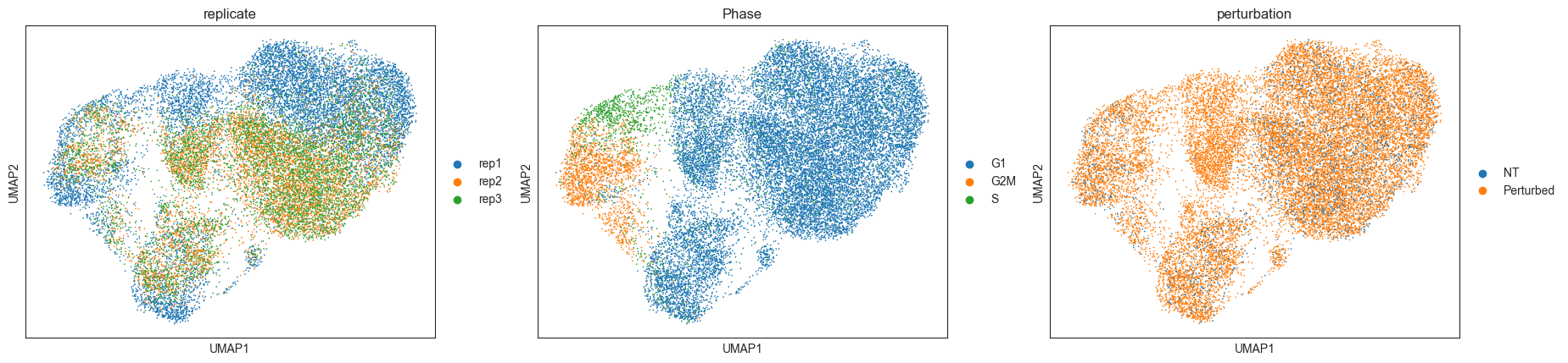
RNA-based clustering is driven by confounding sources of variation

Using the common gene expression-based cell clustering workflow, we expect to discern clusters unique to specific perturbations. Contrary to this, clustering is mainly influenced by cell cycle phases and replicate IDs. The exception is a single cluster, characterized by cells expressing gRNAs related to the IFNgamma pathway.

sc.pp.pca(mdata["rna"])

sc.pp.neighbors(mdata["rna"], metric="cosine")

sc.tl.umap(mdata["rna"])

sc.pl.umap(mdata["rna"], color=["replicate", "Phase", "perturbation"])

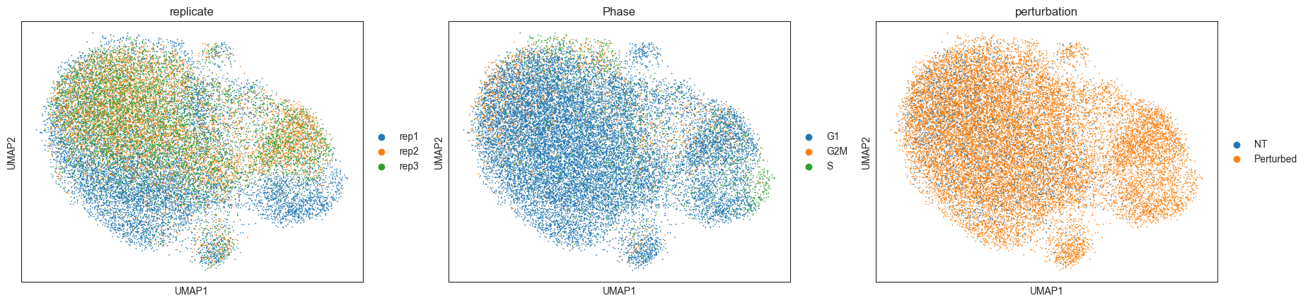
Calculating local perturbation signatures mitigates confounding effects

To regress out the confounding effects, we calculate local perturbation signatures. For each cell, we identify n_neighbors cells from the control pool with the most similar mRNA expression profiles. The perturbation signature is calculated by subtracting the averaged mRNA expression profile of the control neighbors from the mRNA expression profile of each cell.

ms = pt.tl.Mixscape()
ms.perturbation_signature(mdata["rna"], "perturbation", "NT", "replicate")

adata_pert = mdata["rna"].copy()

adata_pert.X = adata_pert.layers["X_pert"]

sc.pp.pca(adata_pert)

sc.pp.neighbors(adata_pert, metric="cosine")

sc.tl.umap(adata_pert)

sc.pl.umap(adata_pert, color=["replicate", "Phase", "perturbation"])

Mixscape identifies cells with no detectable perturbation

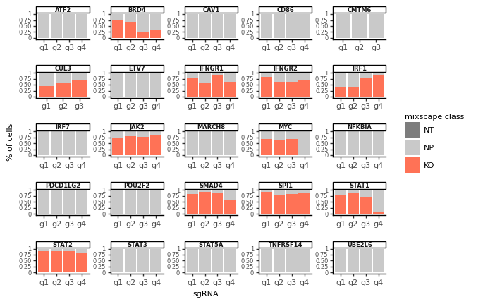
mixscape models each target gene class as a combination of two Gaussian distributions: one for knockout (KO) cells and another for non-perturbed (NP) cells. We assume that NP cells exhibit the same distribution as cells with non-targeting gRNAs (NT). We estimate the KO cell distribution and then compute the posterior probability of a cell belonging to the KO group. Cells with a probability above 0.5 are classified as KOs. This method helped us identify KOs in 11 target gene classes, revealing variations in gRNA targeting efficiency across these classes.

ms.mixscape(adata=mdata["rna"], control="NT", labels="gene_target", layer="X_pert")

We detect variation in gRNA targeting efficiency within each class.

ms.plot_barplot(mdata["rna"], guide_rna_column="NT")

<ggplot: (363011660)>

Inspecting mixscape results

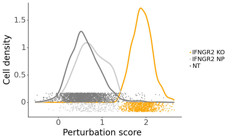
To validate that mixscape accurately assigns perturbation status, we can examine the perturbation score distributions and the posterior probabilities of cells in a specific target gene class, like IFNGR2, comparing these with non-targeting (NT) cells. Additionally, we can conduct differential expression (DE) analyses, demonstrating that reduced expression of IFNG-pathway genes is unique to IFNGR2 KO cells. As an independent verification, we can also assess the PD-L1 protein expression levels in non-perturbed (NP) and knockout (KO) cells for genes known to regulate PD-L1.

ms.plot_perturbscore(adata=mdata["rna"], labels="gene_target", target_gene="IFNGR2", color="orange")

<ggplot: (362586152)>

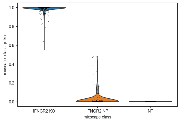
Inspect the posterior probability values in NP and KO cells.

ms.plot_violin(
    adata=mdata["rna"],
    target_gene_idents=["NT", "IFNGR2 NP", "IFNGR2 KO"],
    groupby="mixscape_class",
)

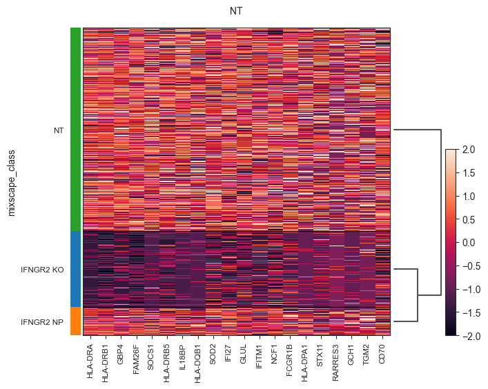
Run DE analysis and visualize results on a heatmap ordering cells by their posterior probability values.

ms.plot_heatmap(
    adata=mdata["rna"],
    labels="gene_target",
    target_gene="IFNGR2",
    layer="X_pert",
    control="NT",
)

WARNING: dendrogram data not found (using key=dendrogram_mixscape_class). Running `sc.tl.dendrogram` with default parameters. For fine tuning it is recommended to run `sc.tl.dendrogram` independently.
WARNING: Groups are not reordered because the `groupby` categories and the `var_group_labels` are different.
categories: IFNGR2 KO, IFNGR2 NP, NT
var_group_labels: NT

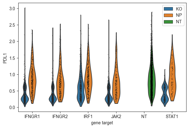
Show that only IFNG pathway KO cells have a reduction in PD-L1 protein expression.

mdata["adt"].obs["mixscape_class_global"] = mdata["rna"].obs["mixscape_class_global"]
ms.plot_violin(
    adata=mdata["adt"],
    target_gene_idents=["NT", "JAK2", "STAT1", "IFNGR1", "IFNGR2", "IRF1"],
    keys="PDL1",
    groupby="gene_target",
    hue="mixscape_class_global",
)

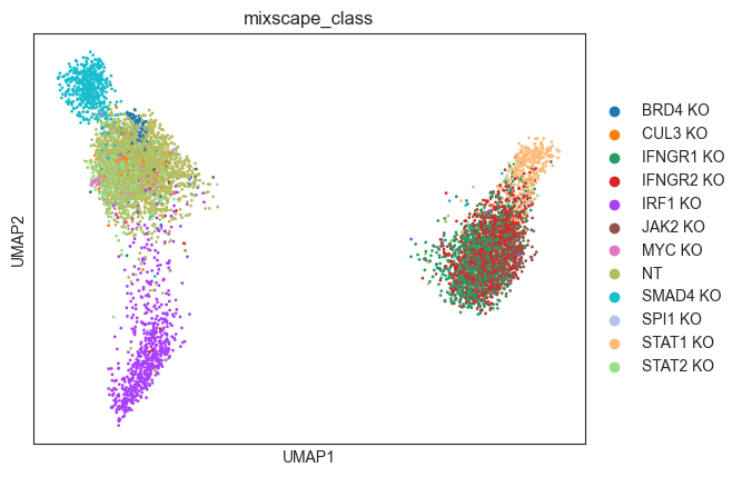
Visualizing perturbation responses with Linear Discriminant Analysis (LDA)

Finally, we use LDA as a dimensionality reduction method to visualize perturbation-specific clusters. LDA tries to maximize the separability of known labels (mixscape classes) using both gene expression and the labels as input.

ms = pt.tl.Mixscape()
ms.lda(adata=mdata["rna"], control="NT", labels="gene_target", layer="X_pert")

ms.plot_lda(adata=mdata["rna"], control="NT")

References

1. Papalexi, E., Mimitou, E.P., Butler, A.W. et al. Characterizing the molecular regulation of inhibitory immune checkpoints with multimodal single-cell screens. Nat Genet 53, 322–331 (2021). https://doi.org/10.1038/s41588-021-00778-2