pertpy.tools.Milo
Methods table
|
Add covariate from cell-level obs to sample-level obs. |
|
Calculates the mean expression in neighbourhoods of each feature. |
|
Assigns a categorical label to neighbourhoods, based on the most frequent label among cells in each neighbourhood. |
|
Assigns a continuous value to neighbourhoods, based on mean cell level covariate stored in adata.obs. |
|
Build graph of neighbourhoods used for visualization of DA results |
|
Builds a sample-level AnnData object storing the matrix of cell counts per sample per neighbourhood. |
|
Performs differential abundance testing on neighbourhoods using QLF test implementation as implemented in edgeR. |
|
Prepare a MuData object for subsequent processing. |
|
Randomly sample vertices on a KNN graph to define neighbourhoods of cells. |
|
Plot beeswarm plot of logFC against nhood labels |
|
Visualize cells in a neighbourhood. |
|
Plot boxplot of cell numbers vs condition of interest. |
|
Visualize DA results on abstracted graph (wrapper around sc.pl.embedding) |
Methods
add_covariate_to_nhoods_var
- Milo.add_covariate_to_nhoods_var(mdata, new_covariates, feature_key='rna')[source]
Add covariate from cell-level obs to sample-level obs. These should be covariates for which a single value can be assigned to each sample.
- Parameters:
- Returns:
None, adds columns to milo_mdata[‘milo’] in place
Examples
>>> import pertpy as pt
>>> import scanpy as sc
>>> adata = pt.dt.bhattacherjee()
>>> milo = pt.tl.Milo()
>>> mdata = milo.load(adata)
>>> sc.pp.neighbors(mdata["rna"])
>>> milo.make_nhoods(mdata["rna"])
>>> mdata = milo.count_nhoods(mdata, sample_col="orig.ident")
>>> milo.add_covariate_to_nhoods_var(mdata, new_covariates=["label"])
add_nhood_expression
- Milo.add_nhood_expression(mdata, layer=None, feature_key='rna')[source]
Calculates the mean expression in neighbourhoods of each feature.
- Parameters:
- Returns:
Updates adata in place to store the matrix of average expression in each neighbourhood in milo_mdata[‘milo’].varm[‘expr’]
Examples
>>> import pertpy as pt
>>> import scanpy as sc
>>> adata = pt.dt.bhattacherjee()
>>> milo = pt.tl.Milo()
>>> mdata = milo.load(adata)
>>> sc.pp.neighbors(mdata["rna"])
>>> milo.make_nhoods(mdata["rna"])
>>> mdata = milo.count_nhoods(mdata, sample_col="orig.ident")
>>> milo.add_nhood_expression(mdata)
annotate_nhoods
- Milo.annotate_nhoods(mdata, anno_col, feature_key='rna')[source]
Assigns a categorical label to neighbourhoods, based on the most frequent label among cells in each neighbourhood. This can be useful to stratify DA testing results by cell types or samples.
- Parameters:
- Returns:
milo_mdata[‘milo’].var[“nhood_annotation”]: assigning a label to each nhood
milo_mdata[‘milo’].var[“nhood_annotation_frac”] stores the fraciton of cells in the neighbourhood with the assigned label
milo_mdata[‘milo’].varm[‘frac_annotation’]: stores the fraction of cells from each label in each nhood
milo_mdata[‘milo’].uns[“annotation_labels”]: stores the column names for milo_mdata[‘milo’].varm[‘frac_annotation’]
- Return type:
None. Adds in place
Examples
>>> import pertpy as pt
>>> import scanpy as sc
>>> adata = pt.dt.bhattacherjee()
>>> milo = pt.tl.Milo()
>>> mdata = milo.load(adata)
>>> sc.pp.neighbors(mdata["rna"])
>>> milo.make_nhoods(mdata["rna"])
>>> mdata = milo.count_nhoods(mdata, sample_col="orig.ident")
>>> milo.annotate_nhoods(mdata, anno_col="cell_type")
annotate_nhoods_continuous
- Milo.annotate_nhoods_continuous(mdata, anno_col, feature_key='rna')[source]
Assigns a continuous value to neighbourhoods, based on mean cell level covariate stored in adata.obs. This can be useful to correlate DA log-foldChanges with continuous covariates such as pseudotime, gene expression scores etc…
- Parameters:
- Returns:
milo_mdata[‘milo’].var[“nhood_{anno_col}”]: assigning a continuous value to each nhood
- Return type:
None. Adds in place
Examples
>>> import pertpy as pt
>>> import scanpy as sc
>>> adata = pt.dt.bhattacherjee()
>>> milo = pt.tl.Milo()
>>> mdata = milo.load(adata)
>>> sc.pp.neighbors(mdata["rna"])
>>> milo.make_nhoods(mdata["rna"])
>>> mdata = milo.count_nhoods(mdata, sample_col="orig.ident")
>>> milo.annotate_nhoods_continuous(mdata, anno_col="nUMI")
build_nhood_graph
- Milo.build_nhood_graph(mdata, basis='X_umap', feature_key='rna')[source]
Build graph of neighbourhoods used for visualization of DA results
- Parameters:
- Returns:
graph of overlap between neighbourhoods (i.e. no of shared cells) - milo_mdata[‘milo’].var[“Nhood_size”]: number of cells in neighbourhoods
- Return type:
milo_mdata[‘milo’].varp[‘nhood_connectivities’]
Examples
>>> import pertpy as pt
>>> import scanpy as sc
>>> adata = pt.dt.bhattacherjee()
>>> milo = pt.tl.Milo()
>>> mdata = milo.load(adata)
>>> sc.pp.neighbors(mdata["rna"])
>>> sc.tl.umap(mdata["rna"])
>>> milo.make_nhoods(mdata["rna"])
>>> mdata = milo.count_nhoods(mdata, sample_col="orig.ident")
>>> milo.build_nhood_graph(mdata)
count_nhoods
- Milo.count_nhoods(data, sample_col, feature_key='rna')[source]
Builds a sample-level AnnData object storing the matrix of cell counts per sample per neighbourhood.
- Parameters:
data (
AnnData|MuData) – AnnData object with neighbourhoods defined in obsm[‘nhoods’] or MuData object with a modality with neighbourhoods defined in obsm[‘nhoods’]sample_col (
str) – Column in adata.obs that contains sample informationfeature_key (
str|None) – If input data is MuData, specify key to cell-level AnnData object. Defaults to ‘rna’.
- Returns:
MuData object storing the original (i.e. rna) AnnData in mudata[feature_key] and the compositional anndata storing the neighbourhood cell counts in mudata[‘milo’]. Here: - mudata[‘milo’].obs_names are samples (defined from adata.obs[‘sample_col’]) - mudata[‘milo’].var_names are neighbourhoods - mudata[‘milo’].X is the matrix counting the number of cells from each sample in each neighbourhood
Examples
>>> import pertpy as pt
>>> import scanpy as sc
>>> adata = pt.dt.bhattacherjee()
>>> milo = pt.tl.Milo()
>>> mdata = milo.load(adata)
>>> sc.pp.neighbors(mdata["rna"])
>>> milo.make_nhoods(mdata["rna"])
>>> mdata = milo.count_nhoods(mdata, sample_col="orig.ident")
da_nhoods
- Milo.da_nhoods(mdata, design, model_contrasts=None, subset_samples=None, add_intercept=True, feature_key='rna', solver='edger')[source]
Performs differential abundance testing on neighbourhoods using QLF test implementation as implemented in edgeR.
- Parameters:
mdata (
MuData) – MuData objectdesign (
str) – Formula for the test, following glm syntax from R (e.g. ‘~ condition’). Terms should be columns in milo_mdata[feature_key].obs.model_contrasts (
str|None) – A string vector that defines the contrasts used to perform DA testing, following glm syntax from R (e.g. “conditionDisease - conditionControl”). If no contrast is specified (default), then the last categorical level in condition of interest is used as the test group. Defaults to None.subset_samples (
list[str] |None) – subset of samples (obs in milo_mdata[‘milo’]) to use for the test. Defaults to None.add_intercept (
bool) – whether to include an intercept in the model. If False, this is equivalent to adding + 0 in the design formula. When model_contrasts is specified, this is set to False by default. Defaults to True.feature_key (
str|None) – If input data is MuData, specify key to cell-level AnnData object. Defaults to ‘rna’.solver (
Literal['edger','batchglm']) – The solver to fit the model to. One of “edger” (requires R, rpy2 and edgeR to be installed) or “batchglm”
- Returns:
logFC stores the log fold change in cell abundance (coefficient from the GLM)
PValue stores the p-value for the QLF test before multiple testing correction
- SpatialFDR stores the p-value adjusted for multiple testing to limit the false discovery rate,
calculated with weighted Benjamini-Hochberg procedure
- Return type:
None, modifies milo_mdata[‘milo’] in place, adding the results of the DA test to .var
Examples
>>> import pertpy as pt
>>> import scanpy as sc
>>> adata = pt.dt.bhattacherjee()
>>> milo = pt.tl.Milo()
>>> mdata = milo.load(adata)
>>> sc.pp.neighbors(mdata["rna"])
>>> milo.make_nhoods(mdata["rna"])
>>> mdata = milo.count_nhoods(mdata, sample_col="orig.ident")
>>> milo.da_nhoods(mdata, design="~label")
load
- Milo.load(input, feature_key='rna')[source]
Prepare a MuData object for subsequent processing.
- Parameters:
- Returns:
MuData object with original AnnData. Defaults to`mudata[feature_key]`.
- Return type:
MuData
Examples
>>> import pertpy as pt
>>> adata = pt.dt.bhattacherjee()
>>> milo = pt.tl.Milo()
>>> mdata = milo.load(adata)
make_nhoods
- Milo.make_nhoods(data, neighbors_key=None, feature_key='rna', prop=0.1, seed=0, copy=False)[source]
Randomly sample vertices on a KNN graph to define neighbourhoods of cells.
The set of neighborhoods get refined by computing the median profile for the neighbourhood in reduced dimensional space and by selecting the nearest vertex to this position. Thus, multiple neighbourhoods may be collapsed to prevent over-sampling the graph space.
- Parameters:
data (
AnnData|MuData) – AnnData object with KNN graph defined in obsp or MuData object with a modality with KNN graph defined in obspneighbors_key (
str|None) – The key in adata.obsp or mdata[feature_key].obsp to use as KNN graph. If not specified, make_nhoods looks .obsp[‘connectivities’] for connectivities (default storage places for scanpy.pp.neighbors). If specified, it looks at .obsp[.uns[neighbors_key][‘connectivities_key’]] for connectivities. Defaults to None.feature_key (
str|None) – If input data is MuData, specify key to cell-level AnnData object. Defaults to ‘rna’.prop (
float) – Fraction of cells to sample for neighbourhood index search. Defaults to 0.1.seed (
int) – Random seed for cell sampling. Defaults to 0.copy (
bool) – Determines whether a copy of the adata is returned. Defaults to False.
- Returns:
If copy=True, returns the copy of adata with the result in .obs, .obsm, and .uns. Otherwise:
nhoods: scipy.sparse._csr.csr_matrix in adata.obsm[‘nhoods’]. A binary matrix of cell to neighbourhood assignments. Neighbourhoods in the columns are ordered by the order of the index cell in adata.obs_names
nhood_ixs_refined: pandas.Series in adata.obs[‘nhood_ixs_refined’]. A boolean indicating whether a cell is an index for a neighbourhood
nhood_kth_distance: pandas.Series in adata.obs[‘nhood_kth_distance’]. The distance to the kth nearest neighbour for each index cell (used for SpatialFDR correction)
nhood_neighbors_key: adata.uns[“nhood_neighbors_key”] KNN graph key, used for neighbourhood construction
Examples
>>> import pertpy as pt
>>> import scanpy as sc
>>> adata = pt.dt.bhattacherjee()
>>> milo = pt.tl.Milo()
>>> mdata = milo.load(adata)
>>> sc.pp.neighbors(mdata["rna"])
>>> milo.make_nhoods(mdata["rna"])
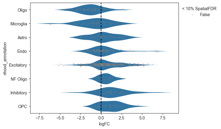
plot_da_beeswarm
- Milo.plot_da_beeswarm(mdata, feature_key='rna', anno_col='nhood_annotation', alpha=0.1, subset_nhoods=None, palette=None, return_fig=None, save=None, show=None)[source]
Plot beeswarm plot of logFC against nhood labels
- Parameters:
mdata (
MuData) – MuData objectanno_col (
str) – Column in adata.uns[‘nhood_adata’].obs to use as annotation. (default: ‘nhood_annotation’.)alpha (
float) – Significance threshold. (default: 0.1)subset_nhoods (
list[str]) – List of nhoods to plot. If None, plot all nhoods. Defaults to None.palette (
str|Sequence[str] |dict[str,str] |None) – Name of Seaborn color palette for violinplots. Defaults to pre-defined category colors for violinplots.
- Return type:
Examples
>>> import pertpy as pt
>>> import scanpy as sc
>>> adata = pt.dt.bhattacherjee()
>>> milo = pt.tl.Milo()
>>> mdata = milo.load(adata)
>>> sc.pp.neighbors(mdata["rna"])
>>> milo.make_nhoods(mdata["rna"])
>>> mdata = milo.count_nhoods(mdata, sample_col="orig.ident")
>>> milo.da_nhoods(mdata, design="~label")
>>> milo.annotate_nhoods(mdata, anno_col="cell_type")
>>> milo.plot_da_beeswarm(mdata)
- Preview:
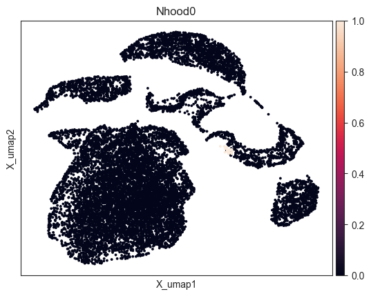
plot_nhood
- Milo.plot_nhood(mdata, ix, feature_key='rna', basis='X_umap', color_map=None, palette=None, return_fig=None, ax=None, show=None, save=None, **kwargs)[source]
Visualize cells in a neighbourhood.
- Parameters:
mdata (
MuData) – MuData object with feature_key slot, storing neighbourhood assignments in mdata[feature_key].obsm[‘nhoods’]ix (
int) – index of neighbourhood to visualizebasis (
str) – Embedding to use for visualization. Defaults to “X_umap”.save (
bool|str|None) – If True or a str, save the figure. A string is appended to the default filename. Infer the filetype if ending on {‘.pdf’, ‘.png’, ‘.svg’}.**kwargs – Additional arguments to scanpy.pl.embedding.
- Return type:
Examples
>>> import pertpy as pt
>>> import scanpy as sc
>>> adata = pt.dt.bhattacherjee()
>>> milo = pt.tl.Milo()
>>> mdata = milo.load(adata)
>>> sc.pp.neighbors(mdata["rna"])
>>> sc.tl.umap(mdata["rna"])
>>> milo.make_nhoods(mdata["rna"])
>>> milo.plot_nhood(mdata, ix=0)
- Preview:
plot_nhood_counts_by_cond
- Milo.plot_nhood_counts_by_cond(mdata, test_var, subset_nhoods=None, log_counts=False, return_fig=None, save=None, show=None)[source]
Plot boxplot of cell numbers vs condition of interest.
- Parameters:
mdata (
MuData) – MuData object storing cell level and nhood level informationtest_var (
str) – Name of column in adata.obs storing condition of interest (y-axis for boxplot)subset_nhoods (
list[str]) – List of obs_names for neighbourhoods to include in plot. If None, plot all nhoods. Defaults to None.log_counts (
bool) – Whether to plot log1p of cell counts. Defaults to False.
- Return type:
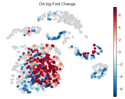
plot_nhood_graph
- Milo.plot_nhood_graph(mdata, alpha=0.1, min_logFC=0, min_size=10, plot_edges=False, title='DA log-Fold Change', color_map=None, palette=None, ax=None, show=None, save=None, **kwargs)[source]
Visualize DA results on abstracted graph (wrapper around sc.pl.embedding)
- Parameters:
mdata (
MuData) – MuData objectalpha (
float) – Significance threshold. (default: 0.1)min_logFC (
float) – Minimum absolute log-Fold Change to show results. If is 0, show all significant neighbourhoods. Defaults to 0.min_size (
int) – Minimum size of nodes in visualization. (default: 10)plot_edges (
bool) – If edges for neighbourhood overlaps whould be plotted. Defaults to False.title (
str) – Plot title. Defaults to “DA log-Fold Change”.save (
bool|str|None) – If True or a str, save the figure. A string is appended to the default filename. Infer the filetype if ending on {‘.pdf’, ‘.png’, ‘.svg’}.**kwargs – Additional arguments to scanpy.pl.embedding.
- Return type:
Examples
>>> import pertpy as pt
>>> import scanpy as sc
>>> adata = pt.dt.bhattacherjee()
>>> milo = pt.tl.Milo()
>>> mdata = milo.load(adata)
>>> sc.pp.neighbors(mdata["rna"])
>>> sc.tl.umap(mdata["rna"])
>>> milo.make_nhoods(mdata["rna"])
>>> mdata = milo.count_nhoods(mdata, sample_col="orig.ident")
>>> milo.da_nhoods(mdata,
>>>            design='~label',
>>>            model_contrasts='labelwithdraw_15d_Cocaine-labelwithdraw_48h_Cocaine')
>>> milo.build_nhood_graph(mdata)
>>> milo.plot_nhood_graph(mdata)
- Preview: