Perturbation Space

The perturbation space departs from the individualistic perspective of cells and instead organizes cells into cohesive ensembles. Every perturbation space summarizes all cells of a perturbation into a single data point, so that we can reason about, compare and combine whole perturbations rather than individual cells.

pertpy offers several distinct ways of determining the perturbation space that will be introduced in this tutorial. We differentiate between perturbation spaces (where we create one data point for all cells of one perturbation) and cluster spaces (where we cluster all cells and then test how well the clustering overlaps with the perturbations).

We will be working with the pre-processed Norman dataset, which encompasses a pooled CRISPR screening experiment comparing the transcriptional effects of overexpressing genes alone or in combination.

Setup

import os

os.environ["KMP_WARNINGS"] = "off"
import warnings

warnings.filterwarnings("ignore")

import pertpy as pt
import scanpy as sc

Dataset

adata = pt.dt.norman_2019()
adata

AnnData object with n_obs × n_vars = 111255 × 19018
    obs: 'guide_identity', 'read_count', 'UMI_count', 'coverage', 'gemgroup', 'good_coverage', 'number_of_cells', 'guide_AHR', 'guide_ARID1A', 'guide_ARRDC3', 'guide_ATL1', 'guide_BAK1', 'guide_BCL2L11', 'guide_BCORL1', 'guide_BPGM', 'guide_C19orf26', 'guide_C3orf72', 'guide_CBFA2T3', 'guide_CBL', 'guide_CDKN1A', 'guide_CDKN1B', 'guide_CDKN1C', 'guide_CEBPA', 'guide_CEBPB', 'guide_CEBPE', 'guide_CELF2', 'guide_CITED1', 'guide_CKS1B', 'guide_CLDN6', 'guide_CNN1', 'guide_CNNM4', 'guide_COL1A1', 'guide_COL2A1', 'guide_CSRNP1', 'guide_DLX2', 'guide_DUSP9', 'guide_EGR1', 'guide_ELMSAN1', 'guide_ETS2', 'guide_FEV', 'guide_FOSB', 'guide_FOXA1', 'guide_FOXA3', 'guide_FOXF1', 'guide_FOXL2', 'guide_FOXO4', 'guide_GLB1L2', 'guide_HES7', 'guide_HK2', 'guide_HNF4A', 'guide_HOXA13', 'guide_HOXB9', 'guide_HOXC13', 'guide_IER5L', 'guide_IGDCC3', 'guide_IKZF3', 'guide_IRF1', 'guide_ISL2', 'guide_JUN', 'guide_KIAA1804', 'guide_KIF18B', 'guide_KIF2C', 'guide_KLF1', 'guide_KMT2A', 'guide_LHX1', 'guide_LYL1', 'guide_MAML2', 'guide_MAP2K3', 'guide_MAP2K6', 'guide_MAP4K3', 'guide_MAP4K5', 'guide_MAP7D1', 'guide_MAPK1', 'guide_MEIS1', 'guide_MIDN', 'guide_NCL', 'guide_NIT1', 'guide_OSR2', 'guide_PLK4', 'guide_POU3F2', 'guide_PRDM1', 'guide_PRTG', 'guide_PTPN1', 'guide_PTPN12', 'guide_PTPN13', 'guide_PTPN9', 'guide_RHOXF2', 'guide_RREB1', 'guide_RUNX1T1', 'guide_S1PR2', 'guide_SAMD1', 'guide_SET', 'guide_SGK1', 'guide_SLC38A2', 'guide_SLC4A1', 'guide_SLC6A9', 'guide_SNAI1', 'guide_SPI1', 'guide_STIL', 'guide_TBX2', 'guide_TBX3', 'guide_TGFBR2', 'guide_TMSB4X', 'guide_TP73', 'guide_TSC22D1', 'guide_UBASH3A', 'guide_UBASH3B', 'guide_ZBTB1', 'guide_ZBTB10', 'guide_ZBTB25', 'guide_ZC3HAV1', 'guide_ZNF318', 'guide_ids', 'n_genes', 'n_genes_by_counts', 'total_counts', 'total_counts_mt', 'pct_counts_mt', 'leiden', 'perturbation_name', 'perturbation_type', 'perturbation_value', 'perturbation_unit'
    var: 'index', 'n_cells', 'mt', 'n_cells_by_counts', 'mean_counts', 'pct_dropout_by_counts', 'total_counts', 'highly_variable', 'means', 'dispersions', 'dispersions_norm'
    uns: 'doi', 'hvg', 'leiden', 'neighbors', 'pca', 'preprocessing_nb_link', 'umap'
    obsm: 'X_pca', 'X_umap'
    varm: 'PCs'
    layers: 'counts'
    obsp: 'connectivities', 'distances'

adata.obs.head()

	guide_identity	read_count	UMI_count	coverage	gemgroup	good_coverage	number_of_cells	guide_AHR	guide_ARID1A	guide_ARRDC3	...	n_genes	n_genes_by_counts	total_counts	total_counts_mt	pct_counts_mt	leiden	perturbation_name	perturbation_type	perturbation_value	perturbation_unit
index
AAACCTGAGAAGAAGC-1	NegCtrl0_NegCtrl0__NegCtrl0_NegCtrl0	1252	67	18.686567	1	True	2	0	0	0	...	4108	4108	19413.0	1327.0	6.835625	10	control	genetic	NaN	NaN
AAACCTGAGGCATGTG-1	TSC22D1_NegCtrl0__TSC22D1_NegCtrl0	2151	104	20.682692	1	True	1	0	0	0	...	3142	3142	13474.0	962.0	7.139676	3	TSC22D1	genetic	NaN	NaN
AAACCTGAGGCCCTTG-1	KLF1_MAP2K6__KLF1_MAP2K6	1037	59	17.576271	1	True	1	0	0	0	...	4229	4229	23228.0	1548.0	6.664371	7	KLF1+MAP2K6	genetic	NaN	NaN
AAACCTGCACGAAGCA-1	NegCtrl10_NegCtrl0__NegCtrl10_NegCtrl0	958	39	24.564103	1	True	1	0	0	0	...	2114	2114	6842.0	523.0	7.643963	2	control	genetic	NaN	NaN
AAACCTGCAGACGTAG-1	CEBPE_RUNX1T1__CEBPE_RUNX1T1	244	14	17.428571	1	True	1	0	0	0	...	2753	2753	9130.0	893.0	9.780942	10	CEBPE+RUNX1T1	genetic	NaN	NaN

5 rows × 123 columns

The Norman dataset has annotations for gene programmes for many perturbations, which we will use later to evaluate the perturbation spaces. These gene programmes can be obtained from the Norman paper:

G1_CYCLE = [
    "CDKN1A",
    {"CDKN1B", "CDKN1A"},
    "CDKN1B",
    {"CDKN1C", "CDKN1A"},
    {"CDKN1C", "CDKN1B"},
    "CDKN1C",
]

ERYTHROID = [
    {"CBL", "CNN1"},
    {"CBL", "PTPN12"},
    {"CBL", "PTPN9"},
    {"CBL", "UBASH3B"},
    {"SAMD1", "PTPN12"},
    {"SAMD1", "UBASH3B"},
    {"UBASH3B", "CNN1"},
    {"UBASH3B", "PTPN12"},
    {"UBASH3B", "PTPN9"},
    {"UBASH3B", "UBASH3A"},
    {"UBASH3B", "ZBTB25"},
    {"BPGM", "SAMD1"},
    "PTPN1",
    {"PTPN12", "PTPN9"},
    {"PTPN12", "UBASH3A"},
    {"PTPN12", "ZBTB25"},
    {"UBASH3A", "CNN1"},
]

PIONEER_FACTORS = [
    {"FOXA1", "FOXF1"},
    {"FOXA1", "FOXL2"},
    {"FOXA1", "HOXB9"},
    {"FOXA3", "FOXA1"},
    {"FOXA3", "FOXF1"},
    {"FOXA3", "FOXL2"},
    {"FOXA3", "HOXB9"},
    "FOXA3",
    {"FOXF1", "FOXL2"},
    {"FOXF1", "HOXB9"},
    {"FOXL2", "MEIS1"},
    "HOXA13",
    "HOXC13",
    {"POU3F2", "FOXL2"},
    "TP73",
    "MIDN",
    {"LYL1", "IER5L"},
    "HOXC13",
    {"DUSP9", "SNAI1"},
    {"ZBTB10", "SNAI1"},
]

GRANULOCYTE_APOPTOSIS = [
    "SPI1",
    "CEBPA",
    {"CEBPB", "CEBPA"},
    "CEBPB",
    {"CEBPE", "CEBPA"},
    {"CEBPE", "CEBPB"},
    {"CEBPE", "RUNX1T1"},
    {"CEBPE", "SPI1"},
    "CEBPE",
    {"ETS2", "CEBPE"},
    {"KLF1", "CEBPA"},
    {"FOSB", "CEBPB"},
    {"FOSB", "CEBPE"},
    {"ZC3HAV1", "CEBPA"},
    {"JUN", "CEBPA"},
]

PRO_GROWTH = [
    {"CEBPE", "KLF1"},
    "KLF1",
    {"KLF1", "BAK1"},
    {"KLF1", "MAP2K6"},
    {"KLF1", "TGFBR2"},
    "ELMSAN1",
    {"MAP2K3", "SLC38A2"},
    {"MAP2K3", "ELMSAN1"},
    "MAP2K3",
    {"MAP2K3", "MAP2K6"},
    {"MAP2K6", "ELMSAN1"},
    "MAP2K6",
    {"MAP2K6", "KLF1"},
]

MEGAKARYOCYTE = [
    {"MAPK1", "TGFBR2"},
    "MAPK1",
    {"ETS2", "MAPK1"},
    "ETS2",
    {"CEBPB", "MAPK1"},
]

programmes = {
    "G1 cell cycle": G1_CYCLE,
    "Erythroid": ERYTHROID,
    "Pioneer factors": PIONEER_FACTORS,
    "Granulocyte apoptosis": GRANULOCYTE_APOPTOSIS,
    "Pro-growth": PRO_GROWTH,
    "Megakaryocyte": MEGAKARYOCYTE,
}

Now we will save the gene programmes in our AnnData object as an additional .obs column:

gene_programme = []

for target_pert in adata.obs["perturbation_name"]:
    if target_pert == "control":
        gene_programme.append("Control")
        continue

    found_programme = False
    for programme, pert_list in programmes.items():
        for pert in pert_list:
            if (isinstance(pert, set) and pert == set(target_pert.split("+"))) or (target_pert == pert):
                gene_programme.append(programme)
                found_programme = True
                break

    if not found_programme:
        gene_programme.append("Unknown")

adata.obs["gene_programme"] = gene_programme

We will work only with the perturbations that have a defined gene programme, since we want to evaluate the perturbation spaces afterward.

adata = adata[adata.obs["gene_programme"] != "Unknown"]

Embed data in Perturbation Spaces

When embedding data in the perturbation space, we aim to generate one data point from all cells of one perturbation. In this tutorial, we introduce several ways to do so:

• Pseudobulk Space

• Discriminator Classifier

• Centroid Space

• Distance Space

• Embedding Space

Pseudobulk Space

The Pseudobulk space returns an Anndata object in which each observation corresponds to the pseudobulk expression of all cells of the respective perturbation.

ps = pt.tl.PseudobulkSpace()
psadata = ps.compute(
    adata,
    target_col="perturbation_name",
    mode="mean",
)

psadata

AnnData object with n_obs × n_vars = 75 × 19018
    obs: 'perturbation_name', 'n_obs_aggregated', 'guide_identity', 'read_count', 'UMI_count', 'coverage', 'gemgroup', 'good_coverage', 'number_of_cells', 'guide_AHR', 'guide_ARID1A', 'guide_ARRDC3', 'guide_ATL1', 'guide_BAK1', 'guide_BCL2L11', 'guide_BCORL1', 'guide_BPGM', 'guide_C19orf26', 'guide_C3orf72', 'guide_CBFA2T3', 'guide_CBL', 'guide_CDKN1A', 'guide_CDKN1B', 'guide_CDKN1C', 'guide_CEBPA', 'guide_CEBPB', 'guide_CEBPE', 'guide_CELF2', 'guide_CITED1', 'guide_CKS1B', 'guide_CLDN6', 'guide_CNN1', 'guide_CNNM4', 'guide_COL1A1', 'guide_COL2A1', 'guide_CSRNP1', 'guide_DLX2', 'guide_DUSP9', 'guide_EGR1', 'guide_ELMSAN1', 'guide_ETS2', 'guide_FEV', 'guide_FOSB', 'guide_FOXA1', 'guide_FOXA3', 'guide_FOXF1', 'guide_FOXL2', 'guide_FOXO4', 'guide_GLB1L2', 'guide_HES7', 'guide_HK2', 'guide_HNF4A', 'guide_HOXA13', 'guide_HOXB9', 'guide_HOXC13', 'guide_IER5L', 'guide_IGDCC3', 'guide_IKZF3', 'guide_IRF1', 'guide_ISL2', 'guide_JUN', 'guide_KIAA1804', 'guide_KIF18B', 'guide_KIF2C', 'guide_KLF1', 'guide_KMT2A', 'guide_LHX1', 'guide_LYL1', 'guide_MAML2', 'guide_MAP2K3', 'guide_MAP2K6', 'guide_MAP4K3', 'guide_MAP4K5', 'guide_MAP7D1', 'guide_MAPK1', 'guide_MEIS1', 'guide_MIDN', 'guide_NCL', 'guide_NIT1', 'guide_OSR2', 'guide_PLK4', 'guide_POU3F2', 'guide_PRDM1', 'guide_PRTG', 'guide_PTPN1', 'guide_PTPN12', 'guide_PTPN13', 'guide_PTPN9', 'guide_RHOXF2', 'guide_RREB1', 'guide_RUNX1T1', 'guide_S1PR2', 'guide_SAMD1', 'guide_SET', 'guide_SGK1', 'guide_SLC38A2', 'guide_SLC4A1', 'guide_SLC6A9', 'guide_SNAI1', 'guide_SPI1', 'guide_STIL', 'guide_TBX2', 'guide_TBX3', 'guide_TGFBR2', 'guide_TMSB4X', 'guide_TP73', 'guide_TSC22D1', 'guide_UBASH3A', 'guide_UBASH3B', 'guide_ZBTB1', 'guide_ZBTB10', 'guide_ZBTB25', 'guide_ZC3HAV1', 'guide_ZNF318', 'guide_ids', 'n_genes', 'n_genes_by_counts', 'total_counts', 'total_counts_mt', 'pct_counts_mt', 'leiden', 'perturbation_type', 'perturbation_value', 'perturbation_unit', 'gene_programme'
    var: 'index', 'n_cells', 'mt', 'n_cells_by_counts', 'mean_counts', 'pct_dropout_by_counts', 'total_counts', 'highly_variable', 'means', 'dispersions', 'dispersions_norm'
    layers: 'mean'

psadata.obs.head()

	perturbation_name	n_obs_aggregated	guide_identity	read_count	UMI_count	coverage	gemgroup	good_coverage	number_of_cells	guide_AHR	...	n_genes	n_genes_by_counts	total_counts	total_counts_mt	pct_counts_mt	leiden	perturbation_type	perturbation_value	perturbation_unit	gene_programme
BAK1+KLF1	BAK1+KLF1	392	KLF1_BAK1__KLF1_BAK1	149	9	16.555556	1	True	2	0	...	3162	3162	11349.0	954.0	8.406027	5	genetic	NaN	NaN	Pro-growth
BPGM+SAMD1	BPGM+SAMD1	300	BPGM_SAMD1__BPGM_SAMD1	1055	58	18.189655	1	True	1	0	...	2991	2991	12677.0	658.0	5.190503	2	genetic	NaN	NaN	Erythroid
CBL+CNN1	CBL+CNN1	348	CBL_CNN1__CBL_CNN1	812	39	20.820513	1	True	1	0	...	2629	2629	10372.0	572.0	5.514847	6	genetic	NaN	NaN	Erythroid
CBL+PTPN9	CBL+PTPN9	305	CBL_PTPN9__CBL_PTPN9	1048	57	18.385965	1	True	1	0	...	1927	1926	6278.0	247.0	3.934374	6	genetic	NaN	NaN	Erythroid
CBL+PTPN12	CBL+PTPN12	333	CBL_PTPN12__CBL_PTPN12	260	12	21.666667	1	True	1	0	...	2883	2883	9445.0	639.0	6.765484	6	genetic	NaN	NaN	Erythroid

5 rows × 125 columns

In the generated AnnData object, each observation represents a perturbation, and its expression is the mode of the PseudobulkSpace function.

Now, the perturbation space can be visualized, and various operations can be applied to analyze it.

sc.pp.neighbors(psadata)
sc.tl.umap(psadata)
sc.pl.umap(psadata, color="perturbation_name")

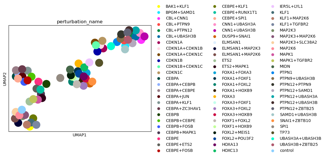
Based on the UMAP visualization of the perturbation space above, we see that the individual perturbations are grouped into clusters. Next, we want to check if the clusters correspond to the gene programmes that we have defined for the individual perturbations above.

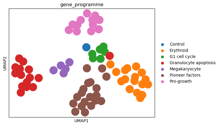
sc.pl.umap(psadata, color="gene_programme")

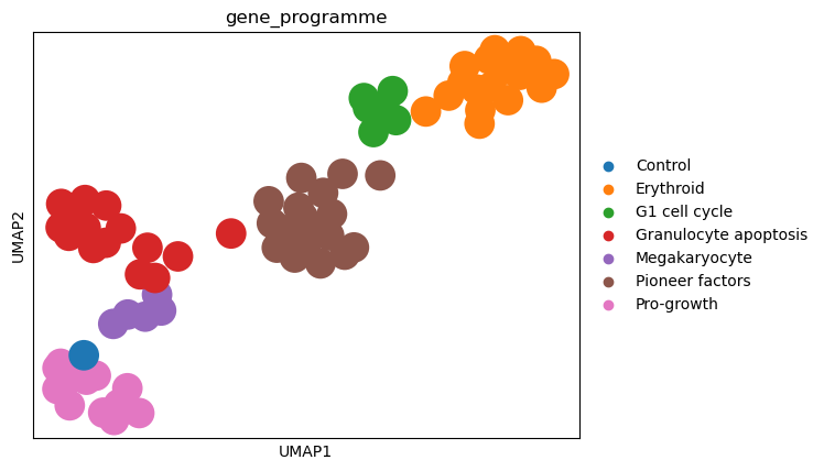
When coloring the individual perturbations according to their gene programs, we observe that the clusters align with the gene programs. This indicates that the perturbation space nicely captures the effects of the perturbations on the cells. Furthermore, when looking at the control perturbation (in the UMAP plot above depicted in blue), we see that it is situated on the periphery of the ‘pro-growth’ cluster, suggesting that the perturbations in this cluster might have only a small effect on the cells.

Another option is to calculate the difference between the perturbations and the control, using the compute_control_diff method. Afterwards, we can again calculate and visualize the perturbation space:

sc.pp.neighbors(adata)
sc.tl.pca(adata)

diff_adata = ps.compute_control_diff(
    adata,
    target_col="perturbation_name",
    reference_key="control",
    embedding_key="X_pca",
)

diff_psadata = ps.compute(diff_adata, target_col="perturbation_name", mode="mean", embedding_key="X_pca")

sc.pp.neighbors(diff_psadata)
sc.tl.umap(diff_psadata)
sc.pl.umap(diff_psadata, color="gene_programme")

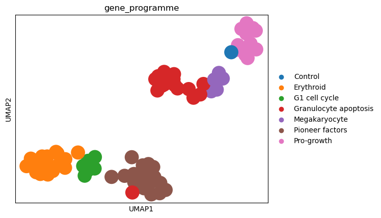
As the individual perturbations already clustered nicely before the control difference was calculated, we do not see a big difference in the UMAP embedding in terms of clustering. We can observe that the perturbations with the same gene programme cluster a bit more densely than before. We also note one “Granulocyte apoptosis” perturbation that is situated in the “Pioneer factors” cluster, which could be worth investigating further.

MLP Classifier Space

The multilayer perceptron (MLP) classifier embedding method trains a neural network based classifier to predict which perturbation has been applied to each cell. Once training has finished, we extract the activations of the penultimate layer for every cell and average them per perturbation, yielding one embedding per perturbation.

ps = pt.tl.MLPClassifierSpace()

Next, we will create and train the model using the compute method. The method accepts different hyperparameters related with the architecture of the model such as hidden_dim, dropout, batch_norm, etc. Training hyperparameters such as batch_size, test_split_size, validation_split_size can also be changed. The compute method trains the model, using the GPU if available, and returns one embedding per perturbation. Each embedding is the averaged penultimate-layer representation of all cells of that perturbation, with a size of 256 as defined by the last entry of hidden_dim.

psadata = ps.compute(
    adata,
    target_col="perturbation_name",
    hidden_dim=[512, 256],
    dropout=0.05,
    batch_size=128,
    batch_norm=True,
    max_epochs=5,
)

An NVIDIA GPU may be present on this machine, but a CUDA-enabled jaxlib is not installed. Falling back to cpu.

psadata.shape

(75, 256)

The psadata object has one observation per perturbation and an embedding of size 256. Because the MLP classifier space already returns perturbation-level embeddings, we can directly visualize and analyze it without any further aggregation.

psadata

AnnData object with n_obs × n_vars = 75 × 256
    obs: 'perturbation_name', 'guide_AHR', 'guide_ARID1A', 'guide_ARRDC3', 'guide_ATL1', 'guide_BAK1', 'guide_BCL2L11', 'guide_BCORL1', 'guide_BPGM', 'guide_C19orf26', 'guide_C3orf72', 'guide_CBFA2T3', 'guide_CBL', 'guide_CDKN1A', 'guide_CDKN1B', 'guide_CDKN1C', 'guide_CEBPA', 'guide_CEBPB', 'guide_CEBPE', 'guide_CELF2', 'guide_CITED1', 'guide_CKS1B', 'guide_CLDN6', 'guide_CNN1', 'guide_CNNM4', 'guide_COL1A1', 'guide_COL2A1', 'guide_CSRNP1', 'guide_DLX2', 'guide_DUSP9', 'guide_EGR1', 'guide_ELMSAN1', 'guide_ETS2', 'guide_FEV', 'guide_FOSB', 'guide_FOXA1', 'guide_FOXA3', 'guide_FOXF1', 'guide_FOXL2', 'guide_FOXO4', 'guide_GLB1L2', 'guide_HES7', 'guide_HK2', 'guide_HNF4A', 'guide_HOXA13', 'guide_HOXB9', 'guide_HOXC13', 'guide_IER5L', 'guide_IGDCC3', 'guide_IKZF3', 'guide_IRF1', 'guide_ISL2', 'guide_JUN', 'guide_KIAA1804', 'guide_KIF18B', 'guide_KIF2C', 'guide_KLF1', 'guide_KMT2A', 'guide_LHX1', 'guide_LYL1', 'guide_MAML2', 'guide_MAP2K3', 'guide_MAP2K6', 'guide_MAP4K3', 'guide_MAP4K5', 'guide_MAP7D1', 'guide_MAPK1', 'guide_MEIS1', 'guide_MIDN', 'guide_NCL', 'guide_NIT1', 'guide_OSR2', 'guide_PLK4', 'guide_POU3F2', 'guide_PRDM1', 'guide_PRTG', 'guide_PTPN1', 'guide_PTPN12', 'guide_PTPN13', 'guide_PTPN9', 'guide_RHOXF2', 'guide_RREB1', 'guide_RUNX1T1', 'guide_S1PR2', 'guide_SAMD1', 'guide_SET', 'guide_SGK1', 'guide_SLC38A2', 'guide_SLC4A1', 'guide_SLC6A9', 'guide_SNAI1', 'guide_SPI1', 'guide_STIL', 'guide_TBX2', 'guide_TBX3', 'guide_TGFBR2', 'guide_TMSB4X', 'guide_TP73', 'guide_TSC22D1', 'guide_UBASH3A', 'guide_UBASH3B', 'guide_ZBTB1', 'guide_ZBTB10', 'guide_ZBTB25', 'guide_ZC3HAV1', 'guide_ZNF318', 'guide_ids', 'perturbation_type', 'gene_programme'

sc.pp.neighbors(psadata, use_rep="X")
sc.tl.umap(psadata)
sc.pl.umap(psadata, color="perturbation_name")

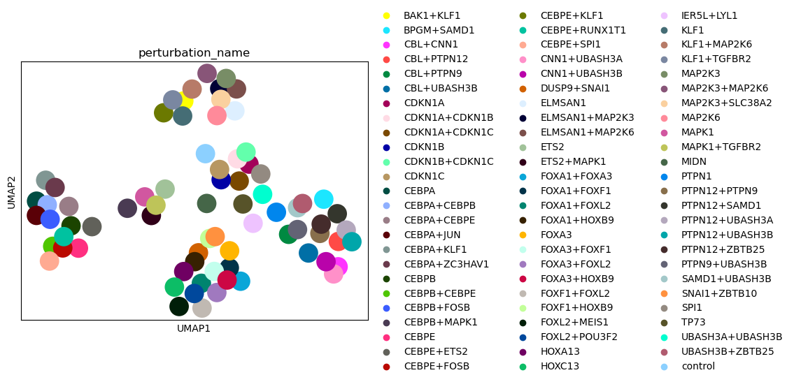
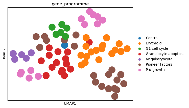
sc.pl.umap(psadata, color="gene_programme")

As we see based on the UMAP plot above, the perturbations are grouped into clusters that correspond to the gene programmes. Importantly, the classifier was not trained to separate the gene programmes, but the individual perturbations. Hence, the fact that the gene programmes are nicely separated in the embedding space indicates that the MLP Classifier works well, as the embeddings capture the effects of the perturbations on the cells.

Logistic Regression Classifier Space

As an alternative to the MLP classifier, we can use a logistic regression classifier to embed the data in the perturbation space. The logistic regression classifier fits one classifier per perturbation and uses the coefficients of the classifier as the embedding for the respective perturbation. Consequently, we obtain one embedding per perturbation, so that we don’t need to calculate a pseudobulk space afterwards, as we did for the MLP classifier. We fit the classifier on PCA data, which was already calculated above.

ps = pt.tl.LRClassifierSpace()
psadata = ps.compute(adata, embedding_key="X_pca", target_col="perturbation_name")
psadata

AnnData object with n_obs × n_vars = 75 × 50
    obs: 'perturbation_name', 'classifier_score', 'guide_AHR', 'guide_ARID1A', 'guide_ARRDC3', 'guide_ATL1', 'guide_BAK1', 'guide_BCL2L11', 'guide_BCORL1', 'guide_BPGM', 'guide_C19orf26', 'guide_C3orf72', 'guide_CBFA2T3', 'guide_CBL', 'guide_CDKN1A', 'guide_CDKN1B', 'guide_CDKN1C', 'guide_CEBPA', 'guide_CEBPB', 'guide_CEBPE', 'guide_CELF2', 'guide_CITED1', 'guide_CKS1B', 'guide_CLDN6', 'guide_CNN1', 'guide_CNNM4', 'guide_COL1A1', 'guide_COL2A1', 'guide_CSRNP1', 'guide_DLX2', 'guide_DUSP9', 'guide_EGR1', 'guide_ELMSAN1', 'guide_ETS2', 'guide_FEV', 'guide_FOSB', 'guide_FOXA1', 'guide_FOXA3', 'guide_FOXF1', 'guide_FOXL2', 'guide_FOXO4', 'guide_GLB1L2', 'guide_HES7', 'guide_HK2', 'guide_HNF4A', 'guide_HOXA13', 'guide_HOXB9', 'guide_HOXC13', 'guide_IER5L', 'guide_IGDCC3', 'guide_IKZF3', 'guide_IRF1', 'guide_ISL2', 'guide_JUN', 'guide_KIAA1804', 'guide_KIF18B', 'guide_KIF2C', 'guide_KLF1', 'guide_KMT2A', 'guide_LHX1', 'guide_LYL1', 'guide_MAML2', 'guide_MAP2K3', 'guide_MAP2K6', 'guide_MAP4K3', 'guide_MAP4K5', 'guide_MAP7D1', 'guide_MAPK1', 'guide_MEIS1', 'guide_MIDN', 'guide_NCL', 'guide_NIT1', 'guide_OSR2', 'guide_PLK4', 'guide_POU3F2', 'guide_PRDM1', 'guide_PRTG', 'guide_PTPN1', 'guide_PTPN12', 'guide_PTPN13', 'guide_PTPN9', 'guide_RHOXF2', 'guide_RREB1', 'guide_RUNX1T1', 'guide_S1PR2', 'guide_SAMD1', 'guide_SET', 'guide_SGK1', 'guide_SLC38A2', 'guide_SLC4A1', 'guide_SLC6A9', 'guide_SNAI1', 'guide_SPI1', 'guide_STIL', 'guide_TBX2', 'guide_TBX3', 'guide_TGFBR2', 'guide_TMSB4X', 'guide_TP73', 'guide_TSC22D1', 'guide_UBASH3A', 'guide_UBASH3B', 'guide_ZBTB1', 'guide_ZBTB10', 'guide_ZBTB25', 'guide_ZC3HAV1', 'guide_ZNF318', 'guide_ids', 'perturbation_type', 'gene_programme'

sc.pp.neighbors(psadata, use_rep="X")
sc.tl.umap(psadata)
sc.pl.umap(psadata, color=["gene_programme"])

Similar to the MLP classifier, the logistic regression classifier also captures the effects of the perturbations on the cells, as the perturbations cluster according to the gene programmes.

Centroid Space

The Centroid Space computes the centroids per perturbation of a pre-computed embedding. Hence, we first need to compute an embedding for the original dataset; here we use UMAP. Note that in this particular dataset, the UMAP is already computed. Nevertheless, we will compute it again to show how to use the Centroid Space in a general setting.

sc.tl.pca(adata)
sc.pp.neighbors(adata)
sc.tl.umap(adata)

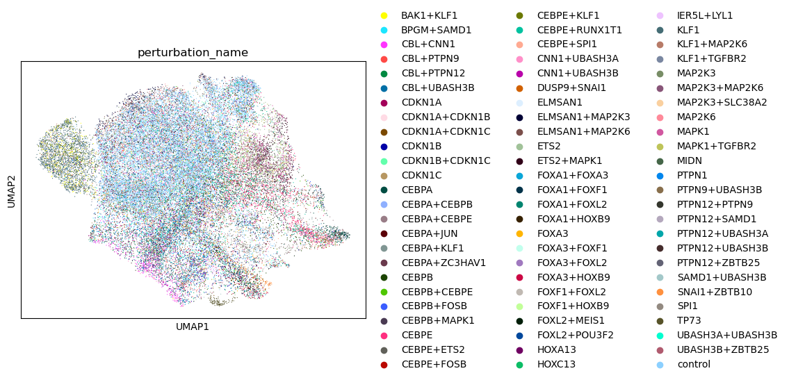
sc.pl.umap(adata, color="perturbation_name")

ps = pt.tl.CentroidSpace()
psadata = ps.compute(adata, target_col="perturbation_name", embedding_key="X_umap")

psadata

AnnData object with n_obs × n_vars = 75 × 2
    obs: 'perturbation_name', 'guide_AHR', 'guide_ARID1A', 'guide_ARRDC3', 'guide_ATL1', 'guide_BAK1', 'guide_BCL2L11', 'guide_BCORL1', 'guide_BPGM', 'guide_C19orf26', 'guide_C3orf72', 'guide_CBFA2T3', 'guide_CBL', 'guide_CDKN1A', 'guide_CDKN1B', 'guide_CDKN1C', 'guide_CEBPA', 'guide_CEBPB', 'guide_CEBPE', 'guide_CELF2', 'guide_CITED1', 'guide_CKS1B', 'guide_CLDN6', 'guide_CNN1', 'guide_CNNM4', 'guide_COL1A1', 'guide_COL2A1', 'guide_CSRNP1', 'guide_DLX2', 'guide_DUSP9', 'guide_EGR1', 'guide_ELMSAN1', 'guide_ETS2', 'guide_FEV', 'guide_FOSB', 'guide_FOXA1', 'guide_FOXA3', 'guide_FOXF1', 'guide_FOXL2', 'guide_FOXO4', 'guide_GLB1L2', 'guide_HES7', 'guide_HK2', 'guide_HNF4A', 'guide_HOXA13', 'guide_HOXB9', 'guide_HOXC13', 'guide_IER5L', 'guide_IGDCC3', 'guide_IKZF3', 'guide_IRF1', 'guide_ISL2', 'guide_JUN', 'guide_KIAA1804', 'guide_KIF18B', 'guide_KIF2C', 'guide_KLF1', 'guide_KMT2A', 'guide_LHX1', 'guide_LYL1', 'guide_MAML2', 'guide_MAP2K3', 'guide_MAP2K6', 'guide_MAP4K3', 'guide_MAP4K5', 'guide_MAP7D1', 'guide_MAPK1', 'guide_MEIS1', 'guide_MIDN', 'guide_NCL', 'guide_NIT1', 'guide_OSR2', 'guide_PLK4', 'guide_POU3F2', 'guide_PRDM1', 'guide_PRTG', 'guide_PTPN1', 'guide_PTPN12', 'guide_PTPN13', 'guide_PTPN9', 'guide_RHOXF2', 'guide_RREB1', 'guide_RUNX1T1', 'guide_S1PR2', 'guide_SAMD1', 'guide_SET', 'guide_SGK1', 'guide_SLC38A2', 'guide_SLC4A1', 'guide_SLC6A9', 'guide_SNAI1', 'guide_SPI1', 'guide_STIL', 'guide_TBX2', 'guide_TBX3', 'guide_TGFBR2', 'guide_TMSB4X', 'guide_TP73', 'guide_TSC22D1', 'guide_UBASH3A', 'guide_UBASH3B', 'guide_ZBTB1', 'guide_ZBTB10', 'guide_ZBTB25', 'guide_ZC3HAV1', 'guide_ZNF318', 'guide_ids', 'perturbation_type', 'gene_programme'
    obsm: 'X_umap'

sc.pl.umap(psadata, color=["perturbation_name", "gene_programme"], legend_loc="on data")

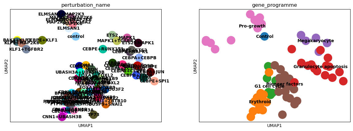
Based on the UMAP plots above, we see that also the Centroid Space is capable of capturing the effects of the perturbations on the cells. The clusters align with the gene programmes, and the control perturbation is situated on the periphery of the ‘Pro-growth’ cluster.

Distance Space

The DistanceSpace represents every perturbation by its statistical distance to all other perturbations, using any metric available in Distance (here the E-distance). The full perturbation-by-perturbation distance matrix is additionally stored in .obsp['distances'], which lets it feed clustering, nearest_perturbations and plot_similarity directly.

ds = pt.tl.DistanceSpace()
ds_adata = ds.compute(adata, target_col="perturbation_name", metric="edistance", embedding_key="X_pca")
ds_adata

AnnData object with n_obs × n_vars = 75 × 75
    obs: 'perturbation_name', 'guide_AHR', 'guide_ARID1A', 'guide_ARRDC3', 'guide_ATL1', 'guide_BAK1', 'guide_BCL2L11', 'guide_BCORL1', 'guide_BPGM', 'guide_C19orf26', 'guide_C3orf72', 'guide_CBFA2T3', 'guide_CBL', 'guide_CDKN1A', 'guide_CDKN1B', 'guide_CDKN1C', 'guide_CEBPA', 'guide_CEBPB', 'guide_CEBPE', 'guide_CELF2', 'guide_CITED1', 'guide_CKS1B', 'guide_CLDN6', 'guide_CNN1', 'guide_CNNM4', 'guide_COL1A1', 'guide_COL2A1', 'guide_CSRNP1', 'guide_DLX2', 'guide_DUSP9', 'guide_EGR1', 'guide_ELMSAN1', 'guide_ETS2', 'guide_FEV', 'guide_FOSB', 'guide_FOXA1', 'guide_FOXA3', 'guide_FOXF1', 'guide_FOXL2', 'guide_FOXO4', 'guide_GLB1L2', 'guide_HES7', 'guide_HK2', 'guide_HNF4A', 'guide_HOXA13', 'guide_HOXB9', 'guide_HOXC13', 'guide_IER5L', 'guide_IGDCC3', 'guide_IKZF3', 'guide_IRF1', 'guide_ISL2', 'guide_JUN', 'guide_KIAA1804', 'guide_KIF18B', 'guide_KIF2C', 'guide_KLF1', 'guide_KMT2A', 'guide_LHX1', 'guide_LYL1', 'guide_MAML2', 'guide_MAP2K3', 'guide_MAP2K6', 'guide_MAP4K3', 'guide_MAP4K5', 'guide_MAP7D1', 'guide_MAPK1', 'guide_MEIS1', 'guide_MIDN', 'guide_NCL', 'guide_NIT1', 'guide_OSR2', 'guide_PLK4', 'guide_POU3F2', 'guide_PRDM1', 'guide_PRTG', 'guide_PTPN1', 'guide_PTPN12', 'guide_PTPN13', 'guide_PTPN9', 'guide_RHOXF2', 'guide_RREB1', 'guide_RUNX1T1', 'guide_S1PR2', 'guide_SAMD1', 'guide_SET', 'guide_SGK1', 'guide_SLC38A2', 'guide_SLC4A1', 'guide_SLC6A9', 'guide_SNAI1', 'guide_SPI1', 'guide_STIL', 'guide_TBX2', 'guide_TBX3', 'guide_TGFBR2', 'guide_TMSB4X', 'guide_TP73', 'guide_TSC22D1', 'guide_UBASH3A', 'guide_UBASH3B', 'guide_ZBTB1', 'guide_ZBTB10', 'guide_ZBTB25', 'guide_ZC3HAV1', 'guide_ZNF318', 'guide_ids', 'perturbation_type', 'gene_programme'
    obsp: 'distances'

Embedding Space

EmbeddingSpace aligns an externally provided per-perturbation embedding (e.g. gene or drug embeddings from foundation models such as scGPT or Geneformer) to the perturbations present in the data. Below we use the pseudobulk representation as a stand-in for such an external embedding to illustrate the mechanics.

import pandas as pd

pseudobulk = pt.tl.PseudobulkSpace().compute(adata, target_col="perturbation_name", mode="mean")
external_embedding = pd.DataFrame(pseudobulk.X, index=pseudobulk.obs_names)
es_adata = pt.tl.EmbeddingSpace().compute(adata, external_embedding, target_col="perturbation_name")
es_adata

AnnData object with n_obs × n_vars = 75 × 19018
    obs: 'perturbation_name', 'guide_AHR', 'guide_ARID1A', 'guide_ARRDC3', 'guide_ATL1', 'guide_BAK1', 'guide_BCL2L11', 'guide_BCORL1', 'guide_BPGM', 'guide_C19orf26', 'guide_C3orf72', 'guide_CBFA2T3', 'guide_CBL', 'guide_CDKN1A', 'guide_CDKN1B', 'guide_CDKN1C', 'guide_CEBPA', 'guide_CEBPB', 'guide_CEBPE', 'guide_CELF2', 'guide_CITED1', 'guide_CKS1B', 'guide_CLDN6', 'guide_CNN1', 'guide_CNNM4', 'guide_COL1A1', 'guide_COL2A1', 'guide_CSRNP1', 'guide_DLX2', 'guide_DUSP9', 'guide_EGR1', 'guide_ELMSAN1', 'guide_ETS2', 'guide_FEV', 'guide_FOSB', 'guide_FOXA1', 'guide_FOXA3', 'guide_FOXF1', 'guide_FOXL2', 'guide_FOXO4', 'guide_GLB1L2', 'guide_HES7', 'guide_HK2', 'guide_HNF4A', 'guide_HOXA13', 'guide_HOXB9', 'guide_HOXC13', 'guide_IER5L', 'guide_IGDCC3', 'guide_IKZF3', 'guide_IRF1', 'guide_ISL2', 'guide_JUN', 'guide_KIAA1804', 'guide_KIF18B', 'guide_KIF2C', 'guide_KLF1', 'guide_KMT2A', 'guide_LHX1', 'guide_LYL1', 'guide_MAML2', 'guide_MAP2K3', 'guide_MAP2K6', 'guide_MAP4K3', 'guide_MAP4K5', 'guide_MAP7D1', 'guide_MAPK1', 'guide_MEIS1', 'guide_MIDN', 'guide_NCL', 'guide_NIT1', 'guide_OSR2', 'guide_PLK4', 'guide_POU3F2', 'guide_PRDM1', 'guide_PRTG', 'guide_PTPN1', 'guide_PTPN12', 'guide_PTPN13', 'guide_PTPN9', 'guide_RHOXF2', 'guide_RREB1', 'guide_RUNX1T1', 'guide_S1PR2', 'guide_SAMD1', 'guide_SET', 'guide_SGK1', 'guide_SLC38A2', 'guide_SLC4A1', 'guide_SLC6A9', 'guide_SNAI1', 'guide_SPI1', 'guide_STIL', 'guide_TBX2', 'guide_TBX3', 'guide_TGFBR2', 'guide_TMSB4X', 'guide_TP73', 'guide_TSC22D1', 'guide_UBASH3A', 'guide_UBASH3B', 'guide_ZBTB1', 'guide_ZBTB10', 'guide_ZBTB25', 'guide_ZC3HAV1', 'guide_ZNF318', 'guide_ids', 'perturbation_type', 'gene_programme'

Cluster Spaces

HDBSCAN Space

HDBSCAN clusters the given data using a hierarchical density-based algorithm. Unlike DBSCAN, it does not require choosing a single density threshold (eps) and can recover clusters of varying density.

You can cluster the data based on the full expression profile stored in .X or on a data representation with reduced dimensionality as specified by the embedding_key parameter. Be aware that computing the clustering on the .X matrix can be very time-consuming for large datasets. In this tutorial, we will use the UMAP embedding, which was already calculated above but will be calculated again in the next cell for the purpose of completeness.

sc.tl.pca(adata, n_comps=15)
sc.pp.neighbors(adata)
sc.tl.umap(adata)

ps = pt.tl.HDBSCANSpace()

hdbscan_psadata = ps.compute(adata, min_cluster_size=50, copy=True, embedding_key="X_umap", n_jobs=2)

sc.pl.umap(hdbscan_psadata, color="hdbscan")

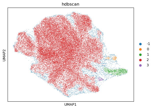
The UMAP plot above shows that several clusters have been identified based on density-based clustering. Of note, one could achieve a finer clustering using the whole data (adata.X) or a different embedding, which we omit here for the sake of simplicity.

Next, we want to evaluate if the identified clusters correspond to the gene programmes that we have defined for the individual perturbations above. Note that the true_label_col specifying the ground truth annotation in the evaluate_clustering method could also be something different from gene programs, or even the perturbation itself. As evaluation metrics, we will calculate the NMI and ARI between the clusters and the gene programmes. Additionally, ASW can be calculated as well but, depending on the size of the dataset, it can take longer to compute.

hdbscan_results = ps.evaluate_clustering(
    hdbscan_psadata,
    true_label_col="gene_programme",
    cluster_col="hdbscan",
    metric="l1",
    metrics=["nmi", "ari"],
)

hdbscan_results

{'nmi': 0.05844213478663895, 'ari': 0.02219895735985616}

The NMI is a value between 0 and 1, where 1 would indicate that the computed clusters perfectly align with the ground truth clusters. A low value indicates that the HDBSCAN clusters computed on the UMAP embedding do not correspond well to the gene programmes. The ARI takes a value between -0.5 and 1, where 0.0 indicates that the clusters are randomly assigned. To improve the clustering, one could run HDBSCAN on higher-dimensional data, e.g. by using a different embedding or no embedding at all.

K-Means Space

Analogous to the steps used for HDBSCAN clustering, we will now use K-means algorithm to cluster the data. This time, we will use the PCA embedding, which we calculated above.

ps = pt.tl.KMeansSpace()
kmeans_psadata = ps.compute(adata, n_clusters=7, copy=True, embedding_key="X_pca")

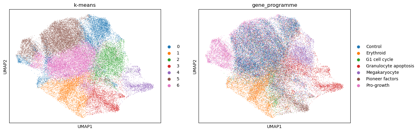
sc.pl.umap(kmeans_psadata, color=["k-means", "gene_programme"])

Again, we will evaluate the calculated clusters using the NMI and ARI metrics:

kmeans_results = ps.evaluate_clustering(
    kmeans_psadata,
    true_label_col="gene_programme",
    cluster_col="k-means",
    metric="l2",
    metrics=["nmi", "ari"],
)

kmeans_results

{'nmi': 0.22106211478938578, 'ari': 0.1543803451401524}

Compared to the NMI and ARI computed for the HDBSCAN clusters, both metrics are higher when using K-means on a PCA embedding. This could be due to the fact that the PCs capture more information than the 2D UMAP embedding, the ability to specify the number of target clusters when running K-means, or simply because K-Means is better suited for this data. Again, one could test using another embedding or no embedding at all, as well as additional parameters to improve the clustering.

Analyzing perturbation spaces

Beyond embedding perturbations, pertpy provides operations that act directly on a perturbation space to compare, relate and combine perturbations.

Perturbation similarity

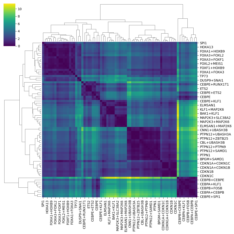
plot_similarity draws a clustered heatmap of the pairwise perturbation distances, reusing the DistanceSpace computed above.

ds.plot_similarity(ds_adata, target_col="perturbation_name")

<seaborn.matrix.ClusterGrid at 0x79e2ec4b6ba0>

Nearest perturbations

Given a perturbation of interest, nearest_perturbations ranks all other perturbations by their proximity in the space, which is useful for discovering perturbations with a similar effect (e.g. a shared mechanism of action). When .obsp['distances'] is present, the precomputed distances are reused directly.

query = ds_adata.obs_names[0]
ds.nearest_perturbations(ds_adata, query, target_col="perturbation_name", n_neighbors=10)

	distance
MAP2K6	0.289199
ELMSAN1	0.313774
MAP2K3	0.470774
MAP2K3+MAP2K6	0.488919
MAP2K3+SLC38A2	0.646155
FOXA3	0.735813
ELMSAN1+MAP2K6	0.768187
CDKN1B	0.908064
UBASH3A+UBASH3B	0.922672
CEBPE+KLF1	1.103267

Combination effects

The Norman dataset contains perturbations of single genes as well as their combinations (named "GENE1+GENE2"). evaluate_combinations compares the additive prediction effect(GENE1) + effect(GENE2) against the measured combination effect (relative to the control). A small distance indicates an additive, non-interacting combination, whereas a large deviation flags a genetic interaction. Adjust reference_key to the control label used in your data.

ps_bulk = pt.tl.PseudobulkSpace().compute(adata, target_col="perturbation_name", mode="mean")
combination_scores = pt.tl.PseudobulkSpace().evaluate_combinations(ps_bulk, reference_key="control", metric="pearson")
combination_scores.head()

	distance	predicted_magnitude	measured_magnitude
CEBPA+CEBPE	0.041895	20.954108	12.621540
CEBPB+MAPK1	0.055697	11.372317	7.239543
CEBPE+SPI1	0.058511	15.732509	14.160367
CEBPE+ETS2	0.058822	10.270707	7.132095
CEBPA+KLF1	0.060676	13.394655	10.591678

Dose response

For dose-resolved screens, dose_response quantifies the effect size of each perturbation as a function of dose by computing the distance of every (perturbation, dose) group to the control. The Norman dataset used above is not dose-resolved, so we load the dose-resolved sci-Plex dataset instead.

sciplex = pt.dt.srivatsan_2020_sciplex2()
sc.pp.normalize_total(sciplex, target_sum=1e4)
sc.pp.log1p(sciplex)
sc.pp.pca(sciplex)

ps = pt.tl.PseudobulkSpace()
ps.dose_response(sciplex, target_col="perturbation", dose_col="dose_value", embedding_key="X_pca")

	perturbation	dose	distance
0	BMS	0.0	14.458705
1	BMS	0.1	16.440267
2	BMS	0.5	19.021279
3	BMS	1.0	15.553012
4	BMS	5.0	17.927020
5	BMS	10.0	18.802652
6	BMS	50.0	1.760868
7	BMS	100.0	0.252982
8	Dex	0.0	13.462214
9	Dex	0.1	13.983747
10	Dex	0.5	14.442097
11	Dex	1.0	15.757915
12	Dex	5.0	14.573900
13	Dex	10.0	15.343917
14	Dex	50.0	14.910395
15	Dex	100.0	14.220436
16	Nutlin	0.0	14.569830
17	Nutlin	0.1	14.341032
18	Nutlin	0.5	14.133695
19	Nutlin	1.0	13.840254
20	Nutlin	5.0	17.403937
21	Nutlin	10.0	18.150556
22	Nutlin	50.0	12.122952
23	Nutlin	100.0	0.012348
24	SAHA	0.0	15.493444
25	SAHA	0.1	16.731112
26	SAHA	0.5	19.180071
27	SAHA	1.0	25.357111
28	SAHA	5.0	23.126392
29	SAHA	10.0	23.113911
30	SAHA	50.0	24.790767
31	SAHA	100.0	20.902018