Differential gene expression#
Differential gene expression (DGE) analysis identifies genes that show statistically significant differences in expression levels across distinct cell populations or conditions. This analysis helps in identifying which cell types are most affected by a condition of interest such as a disease, and characterizing their functional signatures.
Pertpy provides a unified API to several families of DGE models so you can pick the one that fits your design:
Simple statistical tests (
TTest,WilcoxonTest) compare two groups directly on the expression matrix. They are fast, assumption-light, and a reasonable choice when you only have a single binary condition and no covariates to adjust for.Pseudobulk + count-based GLMs (
EdgeR,PyDESeq2) aggregate cells into per-sample pseudobulks and fit a negative-binomial GLM. This is the recommended approach for multi-sample studies with covariates and the current best practice for scRNA-seq DE because it controls false positives caused by treating individual cells as independent replicates.EdgeRcalls into the R package viarpy2;PyDESeq2is a pure-Python reimplementation of DESeq2.Generic linear models (
Statsmodels) wrapstatsmodelsand expose OLS, robust linear models, and GLMs. Use this when your response variable does not look like a count (for example, log-normalised expression or a continuous score).
In the following tutorial we will demonstrate how the edgeR and PyDESeq2 interfaces can be used to model complex interactions using the triple-negative breast cancer (TNBC) Zhang dataset.
Environment setup#
# pip install 'pertpy[de]' decoupler
import warnings

import decoupler as dc
import pertpy as pt
import scanpy as sc

warnings.filterwarnings("ignore")
Dataset#
The Zhang dataset comprises scRNA-seq from 22 patients with advanced TNBC, treated with paclitaxel alone or in combination with the anti-PD-L1 therapy atezolizumab. 78 tumor biopsies and blood samples were collected before treatment (‘pre-treatment’), after treatment (‘post-treatment), and during disease progression (‘progression’). We focused on the transcriptomic data which encompasses approximately 489,490 high-quality immune cells with 27085 measured genes across 99 high resolution cell types.
adata = pt.dt.zhang_2021()
To keep runtimes reasonable and simplify the interpretation, we will only be working with the tissue samples.
adata = adata[adata.obs["Origin"] == "t", :].copy()
adata.obs.head(5)
| Sample | Patient | Origin | Tissue | Efficacy | Group | Treatment | Number of counts | Number of genes | Major celltype | Cluster | |
|---|---|---|---|---|---|---|---|---|---|---|---|
| Cell barcode | |||||||||||
| AAACCTGAGAGTCTGG.Pre_P007_t | Pre_P007_t | P007 | t | lymph_node | PR | Pre-treatment | Anti-PD-L1+Chemo | 2,346 | 748 | T cell | t_Tn-LEF1 |
| AAACCTGAGCACACAG.Pre_P007_t | Pre_P007_t | P007 | t | lymph_node | PR | Pre-treatment | Anti-PD-L1+Chemo | 1,242 | 679 | ILC cell | t_ILC1-IL32 |
| AAACCTGCAAGTCATC.Pre_P007_t | Pre_P007_t | P007 | t | lymph_node | PR | Pre-treatment | Anti-PD-L1+Chemo | 1,593 | 597 | T cell | t_Tn-LEF1 |
| AAACCTGGTTGGGACA.Pre_P007_t | Pre_P007_t | P007 | t | lymph_node | PR | Pre-treatment | Anti-PD-L1+Chemo | 2,404 | 1,203 | T cell | t_CD8_Tem-GZMK |
| AAACCTGTCAGCTCGG.Pre_P007_t | Pre_P007_t | P007 | t | lymph_node | PR | Pre-treatment | Anti-PD-L1+Chemo | 2,034 | 682 | T cell | t_Tn-LEF1 |
When conducting differential gene expression analysis, it is important to understand the dataset well. We will therefore explore the various co-variates first.
adata.obs["Patient"].value_counts()
Patient
P019    37150
P013    22526
P012    14570
P025    14505
P002    10909
P022    10614
P023    10123
P005     8175
P018     7936
P020     7240
P007     7237
P003     4349
P016     4009
P017     4006
P004     3887
P010        8
Name: count, dtype: int64
We remove Patient 10 who has had very few sequenced cells.
adata = adata[~adata.obs["Patient"].isin(["P010"])]
adata.obs["Sample"].value_counts()
Sample
Pre_P019_t     27656
Prog_P013_t    10153
Post_P013_t     9975
Post_P019_t     9494
Post_P025_t     8072
Pre_P022_t      7689
Pre_P012_t      7682
Post_P012_t     6888
Pre_P020_t      6863
Post_P023_t     6813
Pre_P025_t      6433
Post_P018_t     5847
Pre_P002_t      5483
Post_P002_t     5426
Pre_P007_t      4999
Pre_P005_t      4432
Post_P003_t     4349
Pre_P004_t      3887
Pre_P016_t      3862
Post_P005_t     3743
Pre_P023_t      3310
Post_P022_t     2925
Pre_P017_t      2428
Pre_P013_t      2398
Prog_P007_t     2238
Pre_P018_t      2089
Post_P017_t     1578
Post_P020_t      377
Post_P016_t      147
Name: count, dtype: int64
Notably, two samples have less than 1000 sequenced cells. We will not remove them but keep it in mind.
Generally cells can behave quite differently from tissue to tissue. Therefore, it can be useful to conduct DGE tests per tissue and not all tissues jointly. To keep things simple, we will not conduct the tests per tissue separately here.
adata.obs["Tissue"].value_counts()
Tissue
lymph_node    60725
breast        50418
liver         30701
chest_wall    23154
brain          2238
Name: count, dtype: int64
Each patient was treated with a different type of therapy and classified based on efficacy of the treatment as responders (PR: partial response) or non-responders (SD: stable disease, PD: progressive disease).
adata.obs["Treatment"].value_counts()
Treatment
Anti-PD-L1+Chemo    89943
Chemo               77293
Name: count, dtype: int64
adata.obs["Efficacy"].value_counts()
Efficacy
PR    99337
SD    63550
PD     4349
Name: count, dtype: int64
Samples were collected both before and after treatment
adata.obs["Group"].value_counts()
Group
Pre-treatment     89211
Post-treatment    65634
Progression       12391
Name: count, dtype: int64
The dataset was annotated with two levels of cell type annotation:
adata.obs["Major celltype"].value_counts()
Major celltype
T cell          100155
B cell           35588
Myeloid cell     19878
ILC cell         11615
Name: count, dtype: int64
adata.obs["Cluster"].value_counts()
Cluster
t_Tn-LEF1           19046
t_CD8_Tem-GZMK      15371
t_Bmem-CD27         12639
t_CD4_Tcm-LMNA      10886
t_CD8-CXCL13        10689
t_Bn-TCL1A           9695
t_pB-IGHG1           8505
t_CD4_Tact-XIST      8497
t_CD4_Treg-FOXP3     7893
t_CD8_Trm-ZNF683     6456
t_CD4-CXCL13         6282
t_CD8_MAIT-KLRB1     4791
Mix                  4146
t_CD8_Teff-GNLY      3517
t_Bfoc-MKI67         2717
t_Tact-IFI6          2487
t_macro-IL1B         2148
t_macro-IL1RN        1973
t_Bfoc-NEIL1         1865
t_ILC3-AREG          1772
t_mono-FCN1          1684
t_ILC1-VCAM1         1613
t_macro-IGFBP7       1493
t_macro-MGP          1338
t_ILC1-FGFBP2        1309
t_ILC1-SELL          1297
t_ILC1-CD160         1097
t_macro-IFI27        1051
t_macro-TUBA1B       1050
t_ILC1-IL32           972
t_macro-CX3CR1        947
t_ILC2-SPON2          942
t_cDC2-CLEC10A        926
t_macro-MKI67         873
t_ILC1-IFNG           751
t_macro-SPP1          742
t_macro-CCL2          733
t_macro-MMP9          664
t_ILC1-CX3CR1         636
t_mono-S100A89        604
t_macro-CFD           596
t_ILC1-ZNF683         583
t_macro-SLC40A1       577
t_pDC-LILRA4          576
t_macro-FOLR2         491
t_ILC1-GZMK           424
t_cDC1-CLEC9A         273
t_cDC2-FCGR2B         261
t_mast-TPSAB1         250
t_cDC2-CD207          208
t_Bmem-MKI67          167
t_macro-CD24          148
t_mono-SMIM25         139
t_mDC-LAMP3           133
t_ILC3-IL7R           128
t_Tprf-MKI67           94
t_ILC1-CNOT2           91
Name: count, dtype: int64
We remove the Mix cell type analogously to the original publication.
adata = adata[~adata.obs["Cluster"].isin(["Mix"])]
For the remainder of the analysis we will work with the Cluster level because the Major celltype level is not fine-grained enough.
We store the raw counts in a counts layer because most DGE models expect raw counts.
adata.layers["counts"] = adata.X.copy()
Pseudobulks#
To perform DE analysis on our single-cell dataset, we first create pseudobulk samples by aggregating expression counts of cells within each group and sample of interest. This approach allows us to leverage statistical methods originally developed for bulk RNA-seq data, which is the recommended best practice to minimizing false positives in scRNA-seq DE analysis.
For each patient we create 1 pseudobulk sample per cell type by summing up the gene counts within each subpopulation.
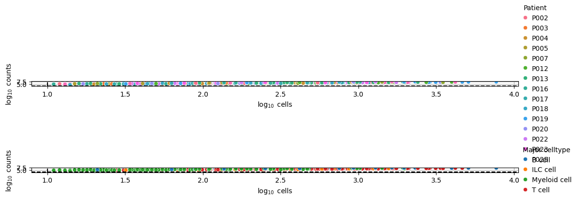
pdata = dc.pp.pseudobulk(adata, sample_col="Patient", groups_col="Cluster", layer="counts", mode="sum")
dc.pp.filter_samples(pdata, inplace=True)
pdata
AnnData object with n_obs × n_vars = 457 × 27085
    obs: 'Patient', 'Cluster', 'Origin', 'Efficacy', 'Treatment', 'Major celltype', 'psbulk_cells', 'psbulk_counts'
    layers: 'psbulk_props'
dc.pl.filter_samples(pdata, groupby=["Patient", "Major celltype"], figsize=(12, 4))
Axes of variation#
The validity of differential gene expression results highly depends on the capture of the major axis of variations in the statistical model. Intermediate data exploration steps such as principal component analysis (PCA) or multidimensional scaling (MDS) on pseudobulk samples allow for the identification of the sources of variation and thus can guide the construction of corresponding design and contrast matrices that model the data.
Now that we have generated the pseudobulk profiles for each patient and each cell type, let’s explore the variability between them. For that, we will first do some simple preprocessing and calculate a PCA.
pdata.layers["counts"] = pdata.X.copy()

sc.pp.normalize_total(pdata, target_sum=1e4)
sc.pp.log1p(pdata)
sc.pp.scale(pdata, max_value=10)
sc.pp.pca(pdata)
# Return raw counts to X
dc.pp.swap_layer(pdata, "counts", inplace=True)
sc.pl.pca(pdata, color=["Patient", "Treatment", "Efficacy", "Cluster"], ncols=1, size=300)
sc.pl.pca_variance_ratio(pdata)
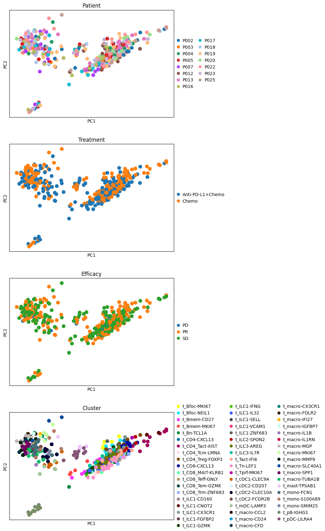
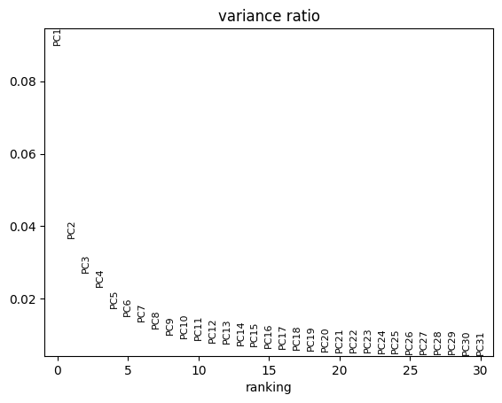
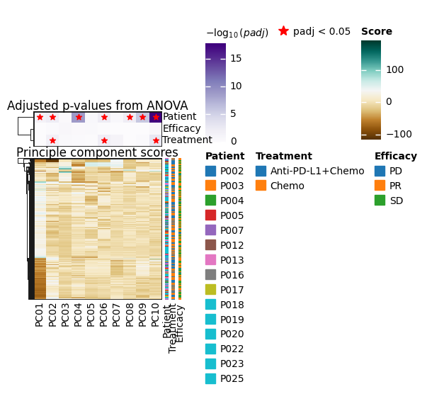
It seems like the four first components explain most of the variance and they easily separate most cell types from one another. In contrast, the principle components do not seem to be associated with Patient, Efficacy or Treatment.
To have a better overview of the association of PCs with sample metadata, let’s perform ANOVA on each PC and see whether they are significantly associated with any technical or biological annotations of our samples
pdata_subset = pdata.copy()
pdata_subset.obs = pdata.obs[["Patient", "Treatment", "Efficacy", "Cluster"]]

dc.tl.rankby_obsm(
    pdata_subset,
    key="X_pca",
    uns_key="pca_anova",
)
dc.pl.obsm(
    pdata_subset,
    key="pca_anova",
    names=["Patient", "Treatment", "Efficacy"],
    titles=["Principle component scores", "Adjusted p-values from ANOVA"],
    cmap_obs={},
)
Differential expression testing with edgeR#
The edger interface further requires edger to be installed in R (BiocManager::install("edgeR")).
A linear model needs a design matrix that encodes, for each sample, the values of the covariates we want to control for or test against. Pertpy lets you describe the design with a Wilkinson formula — the same syntax used by R and patsy. A few examples:
~ Treatment— intercept plus a coefficient per treatment level (the baseline level is absorbed into the intercept).~ Treatment + Efficacy— both covariates as additive, independent effects.~ Treatment + Efficacy + Treatment:Efficacy(equivalently~ Treatment * Efficacy) — additive effects plus an interaction term that asks whether the effect of one covariate depends on the level of the other.
Here we start with the additive model: the type of treatment (Treatment) and response to the treatment (Efficacy) contribute independently to gene expression.
By doing so, we can evaluate:
How much of the variation in gene expression can be attributed to differences in drug efficacy, independent of the type of treatment.
How much of the variation is due to the type of treatment, independent of the efficacy of the drug.
This setup helps in understanding not just whether a treatment works, but how its effectiveness might vary or be influenced by the inherent efficacy of the drug.
edgr = pt.tl.EdgeR(pdata, design="~Efficacy+Treatment")
edgr.fit()
• Calculating NormFactors
• Estimating Dispersions
• Fitting linear model
Fitting the model gave us one coefficient per term in the design.
To turn those coefficients into a biological comparison we evaluate a contrast: a vector with one entry per coefficient that says “take this combination of fitted effects and test whether it differs from zero”.
For a simple two-group comparison along a single column, contrast() builds the right vector automatically.
We will assemble more complex contrasts by hand further down.
res_df = edgr.test_contrasts(edgr.contrast(column="Treatment", baseline="Chemo", group_to_compare="Anti-PD-L1+Chemo"))
res_df.head(10)
| variable | log_fc | logCPM | F | p_value | adj_p_value | contrast | |
|---|---|---|---|---|---|---|---|
| 0 | HBB | 1.165896 | 9.259467 | 494.497680 | 4.767029e-76 | 1.291150e-71 | None |
| 1 | RPS26 | 1.365747 | 10.339090 | 356.827260 | 1.354675e-59 | 1.834569e-55 | None |
| 2 | FDCSP | 4.726368 | 5.455406 | 279.700431 | 1.130304e-52 | 1.020476e-48 | None |
| 3 | IGKV1D-16 | -2.125786 | 5.300726 | 245.219864 | 1.787394e-46 | 1.210289e-42 | None |
| 4 | AZGP1 | -2.878053 | 3.409497 | 168.444076 | 1.330101e-34 | 7.205157e-31 | None |
| 5 | AC135068.2 | -3.971291 | 3.342327 | 159.553825 | 1.426533e-32 | 6.439607e-29 | None |
| 6 | CCL19 | 3.816752 | 4.235494 | 139.161147 | 2.651780e-29 | 1.014408e-25 | None |
| 7 | IGLV5-48 | -4.362628 | 5.474016 | 140.204022 | 2.996222e-29 | 1.014408e-25 | None |
| 8 | HTN1 | 6.556713 | 3.908961 | 162.661491 | 1.031716e-28 | 3.104891e-25 | None |
| 9 | IGHV3-64 | -4.136611 | 4.904814 | 135.687694 | 1.856920e-28 | 5.029468e-25 | None |
The result table has one row per gene. The key columns to look at:
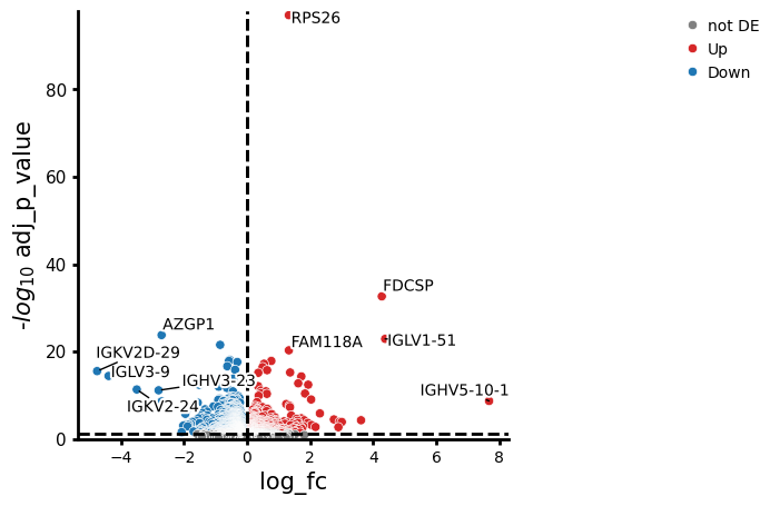
variable— gene symbol.log_fc— log2 fold change between the two contrasted groups. Positive values mean the gene is up ingroup_to_comparerelative tobaseline; negative values mean it is down.p_value— raw p-value from the test thatlog_fcdiffers from zero. Useful for diagnostics, but do not threshold on this directly.adj_p_value— p-value after Benjamini–Hochberg adjustment for multiple testing. This is the value to threshold on (commonly< 0.05).contrast— identifier of the contrast when multiple are tested at once;Nonehere because we only ran one contrast.
A standard summary is “significantly differentially expressed” = adj_p_value < 0.05 and |log_fc| above some effect-size threshold (the volcano plot below uses log2fc_thresh for the latter).
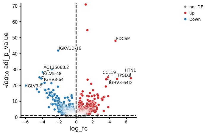
The set of differentially expressed genes can now be used for downstream tasks or as a first step, plotted in a volcano plot.
edgr.plot_volcano(res_df, log2fc_threshold=0)
Once you have a ranked gene table, a typical next step is gene-set / pathway enrichment to turn per-gene statistics into per-pathway statistics.
decoupler integrates well with the result tables produced here.
For example, you can pass the log_fc column from res_df (indexed by variable) into decoupler.mt.ulm together with a prior-knowledge network from OmniPath (collectri(), progeny(), hallmark(), …) to score transcription-factor or pathway activities.
We do not run an enrichment analysis here to keep this tutorial focused on the DE step; decoupler’s bulk functional analysis tutorial is a good starting point.
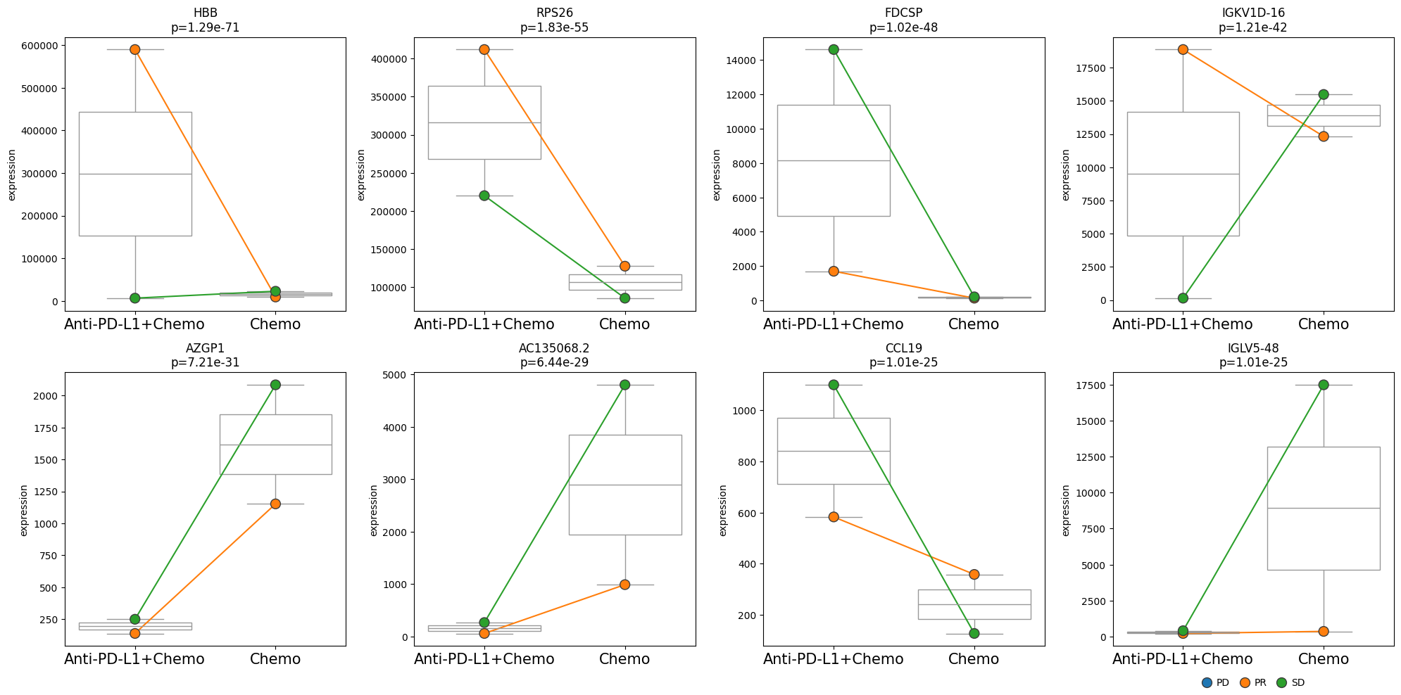
We identified genes that are differentially expressed between the two treatments. Next, we might be interested in looking at the expression levels of these genes across different subgroups. Those subgroups could be different patients or, as in this case, different efficacy groups. For this, we can use the plot_paired function, which enables comparing expression levels between paired samples. Note that the pairing must have been considered in the model design.
edgr.plot_paired(pdata, results_df=res_df, n_top_vars=8, groupby="Treatment", pairedby="Efficacy")
• Performing pseudobulk for paired samples
! 1 unpaired samples removed
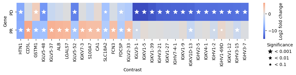
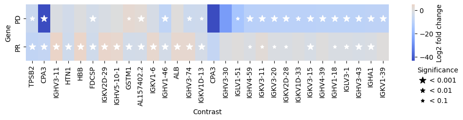
Furthermore, we can also compare the gene expression levels between the different efficacy groups. For this, we use the compare_groups function.
Specifically, we will use the “Stable Disease” (SD) group as the baseline and compare it to the “Partial Response” (PR) and “Progressive Disease” (PD) groups.
res_df = edgr.compare_groups(pdata, column="Efficacy", baseline="SD", groups_to_compare=["PR", "PD"])
edgr.plot_multicomparison_fc(res_df, figsize=(12, 1.5))
• Calculating NormFactors
• Estimating Dispersions
• Fitting linear model
Differential expression testing with PyDESeq2#
The interface of PyDESeq2 in pertpy is very similar.
pds2 = pt.tl.PyDESeq2(adata=pdata, design="~Efficacy+Treatment")
pds2.fit()
Using None as control genes, passed at DeseqDataSet initialization
Fitting size factors...
... done in 0.15 seconds.
Fitting dispersions...
... done in 5.02 seconds.

Fitting dispersion trend curve...
... done in 0.31 seconds.

Fitting MAP dispersions...
... done in 4.52 seconds.

Fitting LFCs...
... done in 5.51 seconds.

Calculating cook's distance...
... done in 0.46 seconds.

Replacing 729 outlier genes.

Fitting dispersions...
... done in 0.17 seconds.

Fitting MAP dispersions...
... done in 0.17 seconds.

Fitting LFCs...
... done in 0.27 seconds.
res_df = pds2.test_contrasts(pds2.contrast(column="Treatment", baseline="Chemo", group_to_compare="Anti-PD-L1+Chemo"))
Log2 fold change & Wald test p-value, contrast vector: [ 0.  0.  0. -1.]
             baseMean  log2FoldChange     lfcSE      stat    pvalue      padj
AL627309.1   0.027626        0.627593  0.428452  1.464793  0.142977       NaN
AL669831.5   0.448998        0.069263  0.199917  0.346458  0.728999  0.853689
FAM87B       0.018980        0.526400  0.594716  0.885128  0.376087       NaN
LINC00115    1.599386       -0.190844  0.119332 -1.599273  0.109760  0.278756
NOC2L       12.462982       -0.086245  0.059518 -1.449061  0.147321  0.338361
...               ...             ...       ...       ...       ...       ...
AP001189.4   0.000000             NaN       NaN       NaN       NaN       NaN
AC011595.1   0.000000             NaN       NaN       NaN       NaN       NaN
TRDJ3        0.000000             NaN       NaN       NaN       NaN       NaN
GOLGA6L1     0.000000             NaN       NaN       NaN       NaN       NaN
AC008569.1   0.000000             NaN       NaN       NaN       NaN       NaN

[27085 rows x 6 columns]
Running Wald tests...
... done in 0.88 seconds.
res_df.head(10)
| variable | baseMean | log_fc | lfcSE | stat | p_value | adj_p_value | contrast | |
|---|---|---|---|---|---|---|---|---|
| 0 | RPS26 | 485.923196 | 1.326838 | 0.061919 | 21.428711 | 7.215009e-102 | 1.013492e-97 | None |
| 1 | FDCSP | 15.211450 | 4.273903 | 0.335305 | 12.746295 | 3.269187e-37 | 2.296114e-33 | None |
| 2 | AZGP1 | 3.718152 | -2.709331 | 0.246142 | -11.007204 | 3.527812e-28 | 1.651839e-24 | None |
| 3 | IGLV1-51 | 83.891787 | 4.380368 | 0.405676 | 10.797710 | 3.528953e-27 | 1.239280e-23 | None |
| 4 | POLR2J3 | 4.443091 | -0.851760 | 0.081243 | -10.484075 | 1.022415e-25 | 2.872371e-22 | None |
| 5 | FAM118A | 15.566632 | 1.327481 | 0.130264 | 10.190700 | 2.181878e-24 | 5.108140e-21 | None |
| 6 | MT-ATP6 | 664.679405 | -0.544051 | 0.056291 | -9.665012 | 4.245693e-22 | 8.519892e-19 | None |
| 7 | NDUFB1 | 44.043809 | 0.768386 | 0.080136 | 9.588463 | 8.940693e-22 | 1.391858e-18 | None |
| 8 | RPS29 | 743.770550 | 0.770006 | 0.080310 | 9.587931 | 8.986940e-22 | 1.391858e-18 | None |
| 9 | HLA-B | 1814.364254 | -0.573257 | 0.059852 | -9.577850 | 9.908580e-22 | 1.391858e-18 | None |
pds2.plot_volcano(res_df, log2fc_threshold=0)
NaNs encountered, dropping rows with NaNs
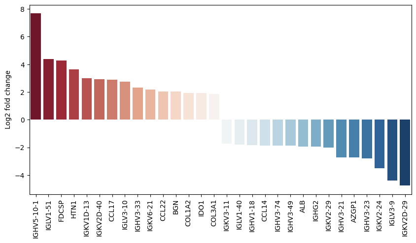
We can also plot the fold changes of the top differentially expressed genes:
pds2.plot_fold_change(res_df, n_top_vars=15)
As already done for edgeR, we can also use PyDESeq2 to compare the gene expression levels between the different efficacy groups.
res_df = pds2.compare_groups(pdata, column="Efficacy", baseline="SD", groups_to_compare=["PR", "PD"])
edgr.plot_multicomparison_fc(res_df, figsize=(12, 1.5))
Using None as control genes, passed at DeseqDataSet initialization
Log2 fold change & Wald test p-value, contrast vector: [ 0.  1. -1.]
             baseMean  log2FoldChange     lfcSE      stat    pvalue      padj
AL627309.1   0.027626       -0.465182  0.648121 -0.717740  0.472918       NaN
AL669831.5   0.448998       -0.385964  0.207275 -1.862088  0.062591  0.290948
FAM87B       0.018980       -0.281550  0.850548 -0.331022  0.740628       NaN
LINC00115    1.599386       -0.253359  0.122537 -2.067623  0.038675  0.226483
NOC2L       12.462982       -0.067935  0.058906 -1.153274  0.248798  0.576505
...               ...             ...       ...       ...       ...       ...
AP001189.4   0.000000             NaN       NaN       NaN       NaN       NaN
AC011595.1   0.000000             NaN       NaN       NaN       NaN       NaN
TRDJ3        0.000000             NaN       NaN       NaN       NaN       NaN
GOLGA6L1     0.000000             NaN       NaN       NaN       NaN       NaN
AC008569.1   0.000000             NaN       NaN       NaN       NaN       NaN

[27085 rows x 6 columns]
Log2 fold change & Wald test p-value, contrast vector: [ 0.  0. -1.]
             baseMean  log2FoldChange     lfcSE      stat    pvalue      padj
AL627309.1   0.027626        0.336716  1.425541  0.236203  0.813276       NaN
AL669831.5   0.448998       -0.205091  0.553761 -0.370360  0.711114       NaN
FAM87B       0.018980        0.544483  1.847643  0.294691  0.768230       NaN
LINC00115    1.599386       -0.224591  0.342215 -0.656288  0.511639  0.673679
NOC2L       12.462982       -0.241951  0.151775 -1.594146  0.110903  0.254624
...               ...             ...       ...       ...       ...       ...
AP001189.4   0.000000             NaN       NaN       NaN       NaN       NaN
AC011595.1   0.000000             NaN       NaN       NaN       NaN       NaN
TRDJ3        0.000000             NaN       NaN       NaN       NaN       NaN
GOLGA6L1     0.000000             NaN       NaN       NaN       NaN       NaN
AC008569.1   0.000000             NaN       NaN       NaN       NaN       NaN

[27085 rows x 6 columns]
Fitting size factors...
... done in 0.17 seconds.
Fitting dispersions...
... done in 3.66 seconds.

Fitting dispersion trend curve...
... done in 0.34 seconds.

Fitting MAP dispersions...
... done in 4.54 seconds.

Fitting LFCs...
... done in 5.96 seconds.

Calculating cook's distance...
... done in 0.52 seconds.

Replacing 763 outlier genes.

Fitting dispersions...
... done in 0.22 seconds.

Fitting MAP dispersions...
... done in 0.22 seconds.

Fitting LFCs...
... done in 0.30 seconds.

Running Wald tests...
... done in 1.33 seconds.
Running Wald tests...
... done in 1.13 seconds.
Model interaction between covariates#
We might be interested in more complex comparisons between patient groups. For example in this study instead of assuming that the type of treatment and its efficacy affect gene expression independently, we can test whether the gene expression changes associated to efficacy might depend on the type of treatment. To do this with a linear model, we model the interaction between the treatment and efficacy, following the syntax from Wilkinson formulas.
# Exclude patient with progressive disease, observed only for one treatment condition
pdata2 = pdata[pdata.obs["Efficacy"] != "PD"].copy()

# Fit DE model with interaction term
pds2 = pt.tl.PyDESeq2(adata=pdata2, design="~ Efficacy + Treatment + Efficacy*Treatment")
pds2.fit()
Using None as control genes, passed at DeseqDataSet initialization
Fitting size factors...
... done in 0.18 seconds.
Fitting dispersions...
... done in 4.47 seconds.

Fitting dispersion trend curve...
... done in 0.37 seconds.

Fitting MAP dispersions...
... done in 5.02 seconds.

Fitting LFCs...
... done in 6.62 seconds.

Calculating cook's distance...
... done in 0.47 seconds.

Replacing 841 outlier genes.

Fitting dispersions...
... done in 0.20 seconds.

Fitting MAP dispersions...
... done in 0.21 seconds.

Fitting LFCs...
... done in 0.27 seconds.
We aim to identify genes that distinguish responders (Efficacy="PR") from non-responders (Efficacy="SD") specifically in patients treated with Anti-PD-L1, but not in those receiving standard chemotherapy. In other words, we want to find genes that are uniquely associated with treatment response in the Anti-PD-L1 group. To do so, we specify a contrast vector using the cond() helper function. This allows you to specify the conditions you want to compare without working out which combination of coefficients in the linear model correspond to your comparison of interest (see here to learn more about contrast vectors and how to build them).
# Specify groups of interest for comparison
interaction_contrast = (
    pds2.cond(Treatment="Anti-PD-L1+Chemo", Efficacy="PR") - pds2.cond(Treatment="Anti-PD-L1+Chemo", Efficacy="SD")
) - (pds2.cond(Treatment="Chemo", Efficacy="PR") - pds2.cond(Treatment="Chemo", Efficacy="SD"))
interaction_contrast
Intercept                            0.0
Efficacy[T.SD]                       0.0
Treatment[T.Chemo]                   0.0
Efficacy[T.SD]:Treatment[T.Chemo]    1.0
Name: 0, dtype: float64
Now we are ready to test for differential expression
interaction_res_df = pds2.test_contrasts(interaction_contrast)
Log2 fold change & Wald test p-value, contrast vector: [0. 0. 0. 1.]
             baseMean  log2FoldChange     lfcSE      stat    pvalue      padj
AL627309.1   0.030299        0.441925  1.259993  0.350736  0.725786       NaN
AL669831.5   0.481510        0.000147  0.421870  0.000349  0.999721  0.999721
FAM87B       0.019790        0.464098  1.709312  0.271511  0.785998       NaN
LINC00115    1.663735        0.444530  0.249670  1.780473  0.074999  0.254101
NOC2L       13.022724        0.441258  0.117724  3.748232  0.000178  0.004734
...               ...             ...       ...       ...       ...       ...
AP001189.4   0.000000             NaN       NaN       NaN       NaN       NaN
AC011595.1   0.000000             NaN       NaN       NaN       NaN       NaN
TRDJ3        0.000000             NaN       NaN       NaN       NaN       NaN
GOLGA6L1     0.000000             NaN       NaN       NaN       NaN       NaN
AC008569.1   0.000000             NaN       NaN       NaN       NaN       NaN

[27085 rows x 6 columns]
Running Wald tests...
... done in 1.01 seconds.
pds2.plot_volcano(interaction_res_df, log2fc_threshold=0)
NaNs encountered, dropping rows with NaNs
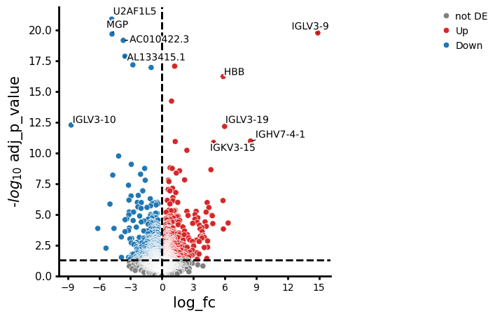
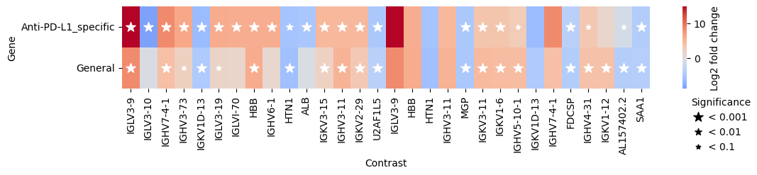
We can also pass several contrasts to test_contrasts, for example to compare DE genes in responders specific to Anti-PD-L1 treatment to responses observed across treatments
general_response_contrast = pds2.cond(Efficacy="PR") - pds2.cond(Efficacy="SD")

interaction_res_df = pds2.test_contrasts(
    {"Anti-PD-L1_specific": interaction_contrast, "General": general_response_contrast}
)

edgr.plot_multicomparison_fc(interaction_res_df, figsize=(12, 1.5))
Log2 fold change & Wald test p-value, contrast vector: [0. 0. 0. 1.]
             baseMean  log2FoldChange     lfcSE      stat    pvalue      padj
AL627309.1   0.030299        0.441925  1.259993  0.350736  0.725786       NaN
AL669831.5   0.481510        0.000147  0.421870  0.000349  0.999721  0.999721
FAM87B       0.019790        0.464098  1.709312  0.271511  0.785998       NaN
LINC00115    1.663735        0.444530  0.249670  1.780473  0.074999  0.254101
NOC2L       13.022724        0.441258  0.117724  3.748232  0.000178  0.004734
...               ...             ...       ...       ...       ...       ...
AP001189.4   0.000000             NaN       NaN       NaN       NaN       NaN
AC011595.1   0.000000             NaN       NaN       NaN       NaN       NaN
TRDJ3        0.000000             NaN       NaN       NaN       NaN       NaN
GOLGA6L1     0.000000             NaN       NaN       NaN       NaN       NaN
AC008569.1   0.000000             NaN       NaN       NaN       NaN       NaN

[27085 rows x 6 columns]
Log2 fold change & Wald test p-value, contrast vector: [ 0. -1.  0.  0.]
             baseMean  log2FoldChange     lfcSE      stat    pvalue      padj
AL627309.1   0.030299       -0.185247  0.869810 -0.212974  0.831347       NaN
AL669831.5   0.481510       -0.375254  0.301541 -1.244454  0.213332  0.458272
FAM87B       0.019790        0.006961  1.181996  0.005889  0.995301       NaN
LINC00115    1.663735       -0.036693  0.181667 -0.201980  0.839932  0.932967
NOC2L       13.022724        0.149331  0.084369  1.769982  0.076730  0.251246
...               ...             ...       ...       ...       ...       ...
AP001189.4   0.000000             NaN       NaN       NaN       NaN       NaN
AC011595.1   0.000000             NaN       NaN       NaN       NaN       NaN
TRDJ3        0.000000             NaN       NaN       NaN       NaN       NaN
GOLGA6L1     0.000000             NaN       NaN       NaN       NaN       NaN
AC008569.1   0.000000             NaN       NaN       NaN       NaN       NaN

[27085 rows x 6 columns]
Running Wald tests...
... done in 1.10 seconds.
Running Wald tests...
... done in 0.98 seconds.