pertpy.tools.Milo#
Methods table#
|
Add covariate from cell-level obs to sample-level obs. |
|
Deprecated alias of |
|
Calculates the mean expression in neighbourhoods of each feature. |
|
Propagate neighbourhood group labels to individual cells. |
|
Assigns a categorical label to neighbourhoods, based on the most frequent label among cells in each neighbourhood. |
|
Assigns a continuous value to neighbourhoods, based on mean cell level covariate stored in adata.obs. |
|
Build graph of neighbourhoods used for visualization of DA results. |
|
Builds a sample-level AnnData object storing the matrix of cell counts per sample per neighbourhood. |
|
Performs differential abundance testing on neighbourhoods using QLF test implementation as implemented in edgeR. |
|
Per-neighbourhood differential expression testing (miloDE). |
|
Find marker genes of neighbourhood groups with pseudobulk differential expression. |
|
Group differentially abundant neighbourhoods into clusters with Louvain community detection. |
|
Prepare a MuData object for subsequent processing. |
|
Randomly sample vertices on a KNN graph to define neighbourhoods of cells. |
|
Plot beeswarm plot of logFC against nhood labels. |
|
Visualize per-neighbourhood DE logFC of a single gene from de_nhoods results. |
|
Visualize cells in a neighbourhood. |
|
Visualize a categorical neighbourhood annotation on the neighbourhood graph. |
|
Plot boxplot of cell numbers vs condition of interest. |
|
Visualize DA results on abstracted graph (wrapper around sc.pl.embedding). |
Methods#
- Milo.add_covariate_to_nhoods_obs(mdata, new_covariates, feature_key='rna')[source]#
Add covariate from cell-level obs to sample-level obs.
These should be covariates for which a single value can be assigned to each sample.
- Parameters:
- Returns:
None, adds columns to milo_mdata[‘milo’] in place
Examples
>>> import pertpy as pt
>>> import scanpy as sc
>>> adata = pt.dt.bhattacherjee()
>>> milo = pt.tl.Milo()
>>> mdata = milo.load(adata)
>>> sc.pp.neighbors(mdata["rna"])
>>> milo.make_nhoods(mdata["rna"])
>>> mdata = milo.count_nhoods(mdata, sample_col="orig.ident")
>>> milo.add_covariate_to_nhoods_obs(mdata, new_covariates=["label"])
- Milo.add_covariate_to_nhoods_var(mdata, new_covariates, feature_key='rna')[source]#
Deprecated alias of
pertpy.tools.Milo.add_covariate_to_nhoods_obs().
- Milo.add_nhood_expression(mdata, layer=None, feature_key='rna')[source]#
Calculates the mean expression in neighbourhoods of each feature.
- Parameters:
- Return type:
- Returns:
Updates adata in place to store the matrix of average expression in each neighbourhood in milo_mdata[‘milo’].varm[‘expr’]
Examples
>>> import pertpy as pt
>>> import scanpy as sc
>>> adata = pt.dt.bhattacherjee()
>>> milo = pt.tl.Milo()
>>> mdata = milo.load(adata)
>>> sc.pp.neighbors(mdata["rna"])
>>> milo.make_nhoods(mdata["rna"])
>>> mdata = milo.count_nhoods(mdata, sample_col="orig.ident")
>>> milo.add_nhood_expression(mdata)
- Milo.annotate_cells_from_nhoods(data, *, feature_key='rna', nhood_group_key='nhood_groups', min_nhoods=1, key_added='nhood_groups')[source]#
Propagate neighbourhood group labels to individual cells.
Each cell is assigned the neighbourhood group it belongs to most often across the neighbourhoods it is part of. Cells in fewer than
min_nhoodslabelled neighbourhoods receive a missing label.- Parameters:
data (
MuData) – MuData with the cell modalityfeature_keyand Milo results indata["milo"].feature_key (
str, default:'rna') – Cell-level modality to annotate.nhood_group_key (
str, default:'nhood_groups') – Column indata["milo"].varwith neighbourhood group labels, as written bygroup_nhoods().min_nhoods (
int, default:1) – Minimum number of labelled neighbourhoods a cell must belong to, to receive a label.key_added (
str, default:'nhood_groups') – Column indata[feature_key].obsto store the per-cell labels.
- Return type:
- Returns:
Nothing, writes
data[feature_key].obs[key_added]in place.
- Milo.annotate_nhoods(mdata, anno_col, feature_key='rna')[source]#
Assigns a categorical label to neighbourhoods, based on the most frequent label among cells in each neighbourhood. This can be useful to stratify DA testing results by cell types or samples.
- Parameters:
- Returns:
Adds in place. - milo_mdata[‘milo’].var[“nhood_annotation”]: assigning a label to each nhood - milo_mdata[‘milo’].var[“nhood_annotation_frac”] stores the fraciton of cells in the neighbourhood with the assigned label - milo_mdata[‘milo’].varm[‘frac_annotation’]: stores the fraction of cells from each label in each nhood - milo_mdata[‘milo’].uns[“annotation_labels”]: stores the column names for milo_mdata[‘milo’].varm[‘frac_annotation’]
Examples
>>> import pertpy as pt
>>> import scanpy as sc
>>> adata = pt.dt.bhattacherjee()
>>> milo = pt.tl.Milo()
>>> mdata = milo.load(adata)
>>> sc.pp.neighbors(mdata["rna"])
>>> milo.make_nhoods(mdata["rna"])
>>> mdata = milo.count_nhoods(mdata, sample_col="orig.ident")
>>> milo.annotate_nhoods(mdata, anno_col="cell_type")
- Milo.annotate_nhoods_continuous(mdata, anno_col, feature_key='rna')[source]#
Assigns a continuous value to neighbourhoods, based on mean cell level covariate stored in adata.obs.
This can be useful to correlate DA log-foldChanges with continuous covariates such as pseudotime, gene expression scores etc…
- Parameters:
- Returns:
Adds in place. - milo_mdata[‘milo’].var[“nhood_{anno_col}”]: assigning a continuous value to each nhood
Examples
>>> import pertpy as pt
>>> import scanpy as sc
>>> adata = pt.dt.bhattacherjee()
>>> milo = pt.tl.Milo()
>>> mdata = milo.load(adata)
>>> sc.pp.neighbors(mdata["rna"])
>>> milo.make_nhoods(mdata["rna"])
>>> mdata = milo.count_nhoods(mdata, sample_col="orig.ident")
>>> milo.annotate_nhoods_continuous(mdata, anno_col="nUMI")
- Milo.build_nhood_graph(mdata, basis='X_umap', feature_key='rna')[source]#
Build graph of neighbourhoods used for visualization of DA results.
- Parameters:
- Returns:
graph of overlap between neighbourhoods (i.e. no of shared cells) - milo_mdata[‘milo’].var[“Nhood_size”]: number of cells in neighbourhoods
- Return type:
milo_mdata[‘milo’].varp[‘nhood_connectivities’]
Examples
>>> import pertpy as pt
>>> import scanpy as sc
>>> adata = pt.dt.bhattacherjee()
>>> milo = pt.tl.Milo()
>>> mdata = milo.load(adata)
>>> sc.pp.neighbors(mdata["rna"])
>>> sc.tl.umap(mdata["rna"])
>>> milo.make_nhoods(mdata["rna"])
>>> mdata = milo.count_nhoods(mdata, sample_col="orig.ident")
>>> milo.build_nhood_graph(mdata)
- Milo.count_nhoods(data, sample_col, feature_key='rna')[source]#
Builds a sample-level AnnData object storing the matrix of cell counts per sample per neighbourhood.
- Parameters:
data (
AnnData|MuData) – AnnData object with neighbourhoods defined in obsm[‘nhoods’] or MuData object with a modality with neighbourhoods defined in obsm[‘nhoods’]sample_col (
str) – Column in adata.obs that contains sample informationfeature_key (
str|None, default:'rna') – If input data is MuData, specify key to cell-level AnnData object.
- Returns:
MuData object storing the original (i.e. rna) AnnData in mudata[feature_key] and the compositional anndata storing the neighbourhood cell counts in mudata[‘milo’]. Here: - mudata[‘milo’].obs_names are samples (defined from adata.obs[‘sample_col’]) - mudata[‘milo’].var_names are neighbourhoods - mudata[‘milo’].X is the matrix counting the number of cells from each sample in each neighbourhood
Examples
>>> import pertpy as pt
>>> import scanpy as sc
>>> adata = pt.dt.bhattacherjee()
>>> milo = pt.tl.Milo()
>>> mdata = milo.load(adata)
>>> sc.pp.neighbors(mdata["rna"])
>>> milo.make_nhoods(mdata["rna"])
>>> mdata = milo.count_nhoods(mdata, sample_col="orig.ident")
- Milo.da_nhoods(mdata, *, design, model_contrasts=None, subset_samples=None, add_intercept=True, feature_key='rna', reml=True, max_iter=50, tol=1e-05, solver='pydeseq2')[source]#
Performs differential abundance testing on neighbourhoods using QLF test implementation as implemented in edgeR.
A random intercept in the design switches to a negative binomial mixed model, which accounts for repeated measurements of the same donor, batch or timepoint instead of treating every sample as independent.
The design must leave residual degrees of freedom, so there have to be more samples than coefficients. Testing one sample per condition raises a ValueError because the dispersion is then not estimable.
- Parameters:
mdata (
MuData) – MuData objectdesign (
str) – Formula for the test, following glm syntax from R (e.g. ‘~ condition’). Terms should be columns in milo_mdata[feature_key].obs. Random intercepts follow the (1 | variable) syntax of R Milo (e.g. ‘~ condition + (1 | donor)’) and fit a mixed model.model_contrasts (
str|None, default:None) – A string vector that defines the contrasts used to perform DA testing, following glm syntax from R (e.g. “conditionDisease - conditionControl”). If no contrast is specified (default), then the last categorical level in condition of interest is used as the test group.subset_samples (
list[str] |None, default:None) – subset of samples (obs in milo_mdata[‘milo’]) to use for the test.add_intercept (
bool, default:True) – whether to include an intercept in the model. If False, this is equivalent to adding + 0 in the design formula. When model_contrasts is specified, this is set to False by default.feature_key (
str|None, default:'rna') – If input data is MuData, specify key to cell-level AnnData object.reml (
bool, default:True) – Whether a mixed model estimates its variance components by restricted maximum likelihood rather than maximum likelihood.max_iter (
int, default:50) – Maximum number of iterations of a mixed model fit.tol (
float, default:1e-05) – Convergence tolerance of a mixed model fit.solver (
Literal['edger','pydeseq2'], default:'pydeseq2') – The solver to fit the model to, ignored for a mixed model. The “edger” solver requires R, rpy2 and edgeR to be installed and is the closest to the R implementation. The “pydeseq2” requires pydeseq2 to be installed. It is still very comparable to the “edger” solver but might be a bit slower.
- Returns:
logFC stores the log fold change in cell abundance (coefficient from the GLM)
PValue stores the p-value for the QLF test before multiple testing correction
- SpatialFDR stores the p-value adjusted for multiple testing to limit the false discovery rate,
calculated with weighted Benjamini-Hochberg procedure
For a mixed model, SE, tvalue, one <variable>_variance per random intercept, Dispersion, Logliklihood and Converged are added as well.
- Return type:
None, modifies milo_mdata[‘milo’] in place, adding the results of the DA test to .var
Examples
>>> import pertpy as pt
>>> import scanpy as sc
>>> adata = pt.dt.bhattacherjee()
>>> milo = pt.tl.Milo()
>>> mdata = milo.load(adata)
>>> sc.pp.neighbors(mdata["rna"])
>>> milo.make_nhoods(mdata["rna"])
>>> mdata = milo.count_nhoods(mdata, sample_col="orig.ident")
>>> milo.da_nhoods(mdata, design="~label")
- Milo.de_nhoods(mdata, design, *, column, baseline, group_to_compare, solver='pydeseq2', layer=None, sample_col=None, feature_key='rna', min_n_cells_per_sample=3, min_count=3, subset_nhoods=None, fit_kwargs=None)[source]#
Per-neighbourhood differential expression testing (miloDE).
For each neighbourhood, cells are pseudobulked by sample and a per-gene linear model is fit on the pseudobulk counts via the existing pertpy DE method (PyDESeq2 or Statsmodels). P-values are corrected twice: across genes within each nhood (BH, exposed as adj_p_value to match pertpy DE conventions) and across nhoods per gene (density-weighted BH, the same correction da_nhoods uses). Neighbourhoods that fail validity checks (too few samples per condition, rank-deficient design) are skipped and marked test_performed=False.
- Parameters:
mdata (
MuData) – MuData with make_nhoods and count_nhoods already run.design (
str) – Right-hand-side formula referencing columns of mdata[feature_key].obs, e.g. “~condition” or “~replicate+condition”.column (
str) – Column from the design that defines the contrast factor.baseline (
str) – Level of column used as the reference (denominator).group_to_compare (
str) – Level of column compared against baseline (numerator).solver (
Literal['pydeseq2','statsmodels'], default:'pydeseq2') – “pydeseq2” for the NB-GLM Wald test, “statsmodels” for OLS by default (pass fit_kwargs={“regression_model”: sm.GLM, “family”: …} for a GLM).layer (
str|None, default:None) – Layer in mdata[feature_key] to use as raw counts; defaults to .X.sample_col (
str|None, default:None) – Column in mdata[feature_key].obs identifying samples; defaults to the value stored by count_nhoods in mdata[‘milo’].uns[‘sample_col’].feature_key (
str|None, default:'rna') – Cell-level modality key in mdata.min_n_cells_per_sample (
int, default:3) – Drop samples with fewer than this many cells in the nhood before pseudobulking.min_count (
int, default:3) – Drop genes whose total pseudobulk count across the surviving samples is below this threshold.subset_nhoods (
list[int] |None, default:None) – Optional integer indices (into mdata[‘milo’].var_names) restricting which nhoods are tested.fit_kwargs (
dict|None, default:None) – Extra keyword arguments forwarded to the per-nhood model’s fit.
- Return type:
- Returns:
Long-form DataFrame with one row per (nhood, gene) pair, columns nhood, variable, log_fc, p_value, adj_p_value, pval_corrected_across_nhoods, test_performed. Skipped nhoods contribute rows with NaN test statistics and test_performed=False.
Examples
>>> import pertpy as pt
>>> import scanpy as sc
>>> adata = pt.dt.bhattacherjee()
>>> milo = pt.tl.Milo()
>>> mdata = milo.load(adata)
>>> sc.pp.neighbors(mdata["rna"])
>>> milo.make_nhoods(mdata["rna"])
>>> mdata = milo.count_nhoods(mdata, sample_col="orig.ident")
>>> de = milo.de_nhoods(
...     mdata, design="~label", column="label", baseline="control", group_to_compare="treated"
... )
- Milo.find_nhood_group_markers(data, *, group_to_compare=None, baseline=None, nhood_group_key='nhood_groups', sample_col='sample', covariates=None, feature_key='rna', layer=None, n_top_genes=None, var_names=None, solver='pydeseq2')[source]#
Find marker genes of neighbourhood groups with pseudobulk differential expression.
Cells are aggregated into pseudobulk samples per (
sample_col,nhood_group_key) combination and tested for differential expression between groups, reusing pertpy’sPyDESeq2andEdgeRmethods. With bothgroup_to_compareandbaselinea single two-group contrast is run, otherwise each group is tested against all others. Neighbourhood group labels are expected at the cell level, as written byannotate_cells_from_nhoods().- Parameters:
data (
AnnData|MuData) – AnnData, or the MuData holding the cell modalityfeature_key.group_to_compare (
str|None, default:None) – Group to test in a two-group contrast; must be a level ofnhood_group_key.baseline (
str|None, default:None) – Reference group in a two-group contrast; must be a level ofnhood_group_key.nhood_group_key (
str, default:'nhood_groups') – Column in.obswith per-cell neighbourhood group labels; cells with missing labels are dropped.sample_col (
str, default:'sample') – Column in.obsidentifying the samples to pseudobulk over.covariates (
Collection[str] |None, default:None) – Additional.obscolumns to include in the design formula.feature_key (
str, default:'rna') – Modality to use whendatais a MuData.layer (
str|None, default:None) – Layer with raw counts to aggregate;Xis used if None.n_top_genes (
int|None, default:None) – If given, restrict testing to this many highly variable genes.var_names (
Collection[str] |None, default:None) – If given, restrict testing to these genes; overridesn_top_genes.solver (
Literal['pydeseq2','edger'], default:'pydeseq2') – Differential expression backend,"pydeseq2"or"edger".
- Return type:
- Returns:
A
DataFramewith one row per gene and columnsvariable,log_fc,p_valueandadj_p_value, plus agroupcolumn when testing one-vs-rest.
Examples
>>> import pertpy as pt
>>> import scanpy as sc
>>> adata = pt.dt.bhattacherjee()
>>> milo = pt.tl.Milo()
>>> mdata = milo.load(adata)
>>> sc.pp.neighbors(mdata["rna"])
>>> milo.make_nhoods(mdata["rna"])
>>> mdata = milo.count_nhoods(mdata, sample_col="orig.ident")
>>> milo.da_nhoods(mdata, design="~label")
>>> milo.build_nhood_graph(mdata)
>>> milo.group_nhoods(mdata)
>>> milo.annotate_cells_from_nhoods(mdata)
>>> markers = milo.find_nhood_group_markers(mdata, sample_col="orig.ident")
- Milo.group_nhoods(data, *, feature_key='milo', da_fdr=0.1, overlap=1, max_lfc_delta=None, merge_discord=False, subset_nhoods=None, key_added='nhood_groups')[source]#
Group differentially abundant neighbourhoods into clusters with Louvain community detection.
This is a Python re-implementation of miloR’s
groupNhoods. All neighbourhoods are clustered on the neighbourhood graph in.varp["nhood_connectivities"](built bybuild_nhood_graph()) with Louvain community detection. Beforehand, edges between differentially abundant neighbourhoods (SpatialFDR < da_fdr) with discordant logFC signs are removed, and edges are optionally filtered by shared-cell overlap and logFC difference. Group labels are written to.var[key_added], with missing labels only for neighbourhoods excluded bysubset_nhoods.Requires the optional GPL-licensed
igraphpackage.- Parameters:
data (
AnnData|MuData) – AnnData with Milo results, or the MuData holding modalityfeature_key.feature_key (
str, default:'milo') – Modality to use whendatais a MuData.da_fdr (
float, default:0.1) – SpatialFDR threshold below which neighbourhoods are considered differentially abundant.overlap (
int, default:1) – Minimum number of shared cells for an edge between two neighbourhoods to be kept.max_lfc_delta (
float|None, default:None) – If given, drop edges between neighbourhoods whose logFC differs by more than this.merge_discord (
bool, default:False) – If False, drop edges between differentially abundant neighbourhoods with opposite logFC signs.subset_nhoods (
Series|ndarray|Sequence[int] |Sequence[str] |None, default:None) – Restrict clustering to these neighbourhoods (boolean mask, integer indices, or names).key_added (
str, default:'nhood_groups') – Column in.varto store the group labels.
- Return type:
- Returns:
Nothing, writes
.var[key_added]in place.
Examples
>>> import pertpy as pt
>>> import scanpy as sc
>>> adata = pt.dt.bhattacherjee()
>>> milo = pt.tl.Milo()
>>> mdata = milo.load(adata)
>>> sc.pp.neighbors(mdata["rna"])
>>> milo.make_nhoods(mdata["rna"])
>>> mdata = milo.count_nhoods(mdata, sample_col="orig.ident")
>>> milo.da_nhoods(mdata, design="~label")
>>> milo.build_nhood_graph(mdata)
>>> milo.group_nhoods(mdata)
- Milo.load(input, feature_key='rna')[source]#
Prepare a MuData object for subsequent processing.
- Parameters:
- Return type:
- Returns:
mudata.MuDataobject with original AnnData.
Examples
>>> import pertpy as pt
>>> adata = pt.dt.bhattacherjee()
>>> milo = pt.tl.Milo()
>>> mdata = milo.load(adata)
- Milo.make_nhoods(data, *, neighbors_key=None, feature_key='rna', prop=0.1, seed=0, copy=False)[source]#
Randomly sample vertices on a KNN graph to define neighbourhoods of cells.
The set of neighborhoods get refined by computing the median profile for the neighbourhood in reduced dimensional space and by selecting the nearest vertex to this position. Thus, multiple neighbourhoods may be collapsed to prevent over-sampling the graph space.
- Parameters:
data (
AnnData|MuData) – AnnData object with KNN graph defined in obsp or MuData object with a modality with KNN graph defined in obspneighbors_key (
str|None, default:None) – The key in adata.obsp or mdata[feature_key].obsp to use as KNN graph. If not specified, make_nhoods looks at .obsp[‘connectivities’] for connectivities. If specified, looks at .obsp[neighbors_key + ‘_connectivities’] for connectivities.feature_key (
str|None, default:'rna') – If input data is MuData, specify key to cell-level AnnData object.prop (
float, default:0.1) – Fraction of cells to sample for neighbourhood index search.seed (
int, default:0) – Random seed for cell sampling.copy (
bool, default:False) – Determines whether a copy of the adata is returned.
- Returns:
If copy=True, returns the copy of adata with the result in .obs, .obsm, and .uns. Otherwise:
nhoods:
scipy.sparse.csr_matrixin adata.obsm[‘nhoods’]. A binary matrix of cell to neighbourhood assignments. Neighbourhoods in the columns are ordered by the order of the index cell in adata.obs_namesnhood_ixs_refined: pandas.Series in adata.obs[‘nhood_ixs_refined’]. A boolean indicating whether a cell is an index for a neighbourhood
nhood_kth_distance: pandas.Series in adata.obs[‘nhood_kth_distance’]. The distance to the kth nearest neighbour for each index cell (used for SpatialFDR correction)
nhood_neighbors_key: adata.uns[“nhood_neighbors_key”] KNN graph key, used for neighbourhood construction
Examples
>>> import pertpy as pt
>>> import scanpy as sc
>>> adata = pt.dt.bhattacherjee()
>>> milo = pt.tl.Milo()
>>> mdata = milo.load(adata)
>>> sc.pp.neighbors(mdata["rna"])
>>> milo.make_nhoods(mdata["rna"])
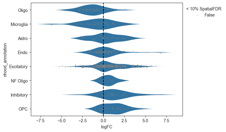
- Milo.plot_da_beeswarm(mdata, *, feature_key='rna', anno_col='nhood_annotation', padj_threshold=0.1, subset_nhoods=None, palette=None, return_fig=False, alpha=None)[source]#
Plot beeswarm plot of logFC against nhood labels.
- Parameters:
mdata (
MuData) – MuData objectfeature_key (
str|None, default:'rna') – Key in mdata to the cell-level AnnData object.anno_col (
str, default:'nhood_annotation') – Column in adata.uns[‘nhood_adata’].obs to use as annotation. (default: ‘nhood_annotation’.)padj_threshold (
float, default:0.1) – Significance threshold. (default: 0.1)subset_nhoods (
list[str] |None, default:None) – List of nhoods to plot. If None, plot all nhoods.palette (
str|Sequence[str] |dict[str,str] |None, default:None) – Name of Seaborn color palette for violinplots. Defaults to pre-defined category colors for violinplots.alpha (
float|None, default:None) – Deprecated and will be removed in a future release. Use padj_threshold.return_fig (
bool, default:False) – if True, returns figure of the plot, that can be used for saving.
- Return type:
- Returns:
If return_fig is True, returns the figure, otherwise None.
Examples
>>> import pertpy as pt
>>> import scanpy as sc
>>> adata = pt.dt.bhattacherjee()
>>> milo = pt.tl.Milo()
>>> mdata = milo.load(adata)
>>> sc.pp.neighbors(mdata["rna"])
>>> milo.make_nhoods(mdata["rna"])
>>> mdata = milo.count_nhoods(mdata, sample_col="orig.ident")
>>> milo.da_nhoods(mdata, design="~label")
>>> milo.annotate_nhoods(mdata, anno_col="cell_type")
>>> milo.plot_da_beeswarm(mdata)
- Preview:
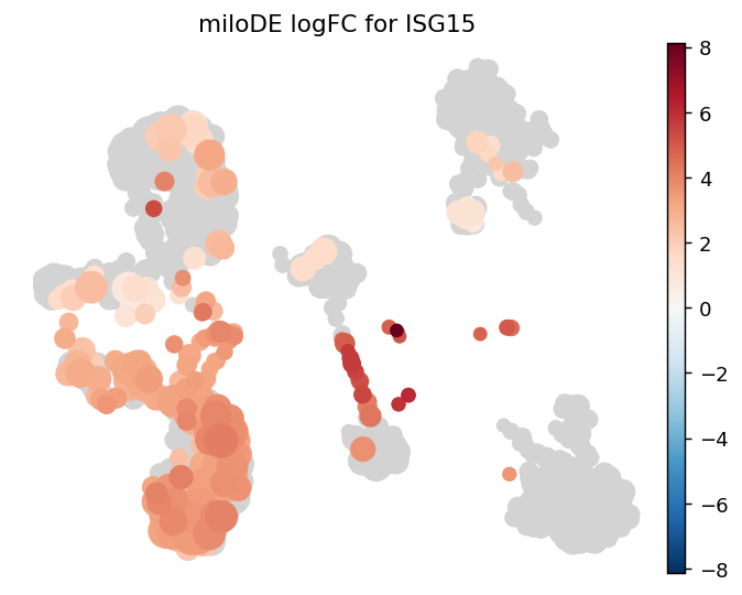
- Milo.plot_de_nhood_graph(mdata, de_results, gene, *, padj_threshold=0.1, min_logFC=0, min_size=10, plot_edges=False, title=None, color_map=None, palette=None, ax=None, return_fig=False, **kwargs)[source]#
Visualize per-neighbourhood DE logFC of a single gene from de_nhoods results.
Pairs with de_nhoods the same way plot_nhood_graph pairs with da_nhoods. Uses the same embedding (build_nhood_graph must have been run) and colors nhoods by log_fc, masking those with pval_corrected_across_nhoods > padj_threshold.
- Parameters:
mdata (
MuData) – MuData with build_nhood_graph already run.de_results (
DataFrame) – Long DataFrame returned by de_nhoods.gene (
str) – Gene to plot; must appear in de_results[“variable”].padj_threshold (
float, default:0.1) – Significance threshold on pval_corrected_across_nhoods.min_logFC (
float, default:0) – Minimum absolute log fold-change to color a nhood.min_size (
int, default:10) – Multiplier on Nhood_size for the node radius.plot_edges (
bool, default:False) – Whether to draw nhood overlap edges.title (
str|None, default:None) – Plot title; defaults to miloDE logFC for <gene>.return_fig (
bool, default:False) – if True, returns figure of the plot, that can be used for saving.**kwargs – Forwarded to scanpy.pl.embedding.
- Return type:
Examples
>>> import pertpy as pt
>>> import scanpy as sc
>>> adata = pt.dt.bhattacherjee()
>>> milo = pt.tl.Milo()
>>> mdata = milo.load(adata)
>>> sc.pp.neighbors(mdata["rna"])
>>> sc.tl.umap(mdata["rna"])
>>> milo.make_nhoods(mdata["rna"])
>>> mdata = milo.count_nhoods(mdata, sample_col="orig.ident")
>>> milo.build_nhood_graph(mdata)
>>> de = milo.de_nhoods(
...     mdata,
...     design="~label",
...     column="label",
...     baseline="control",
...     group_to_compare="treated",
...     layer="counts",
... )
>>> milo.plot_de_nhood_graph(mdata, de, gene="CD4")
- Preview:
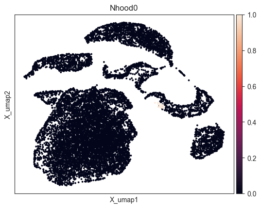
- Milo.plot_nhood(mdata, ix, *, feature_key='rna', basis='X_umap', color_map=None, palette=None, ax=None, return_fig=False, **kwargs)[source]#
Visualize cells in a neighbourhood.
- Parameters:
mdata (
MuData) – MuData object with feature_key slot, storing neighbourhood assignments in mdata[feature_key].obsm[‘nhoods’]ix (
int) – index of neighbourhood to visualizefeature_key (
str|None, default:'rna') – Key in mdata to the cell-level AnnData object.basis (
str, default:'X_umap') – Embedding to use for visualization.color_map (
Colormap|str|None, default:None) – Colormap to use for coloring.palette (
str|Sequence[str] |None, default:None) – Color palette to use for coloring.return_fig (
bool, default:False) – if True, returns figure of the plot, that can be used for saving.**kwargs – Additional arguments to scanpy.pl.embedding.
- Return type:
Examples
>>> import pertpy as pt
>>> import scanpy as sc
>>> adata = pt.dt.bhattacherjee()
>>> milo = pt.tl.Milo()
>>> mdata = milo.load(adata)
>>> sc.pp.neighbors(mdata["rna"])
>>> sc.tl.umap(mdata["rna"])
>>> milo.make_nhoods(mdata["rna"])
>>> milo.plot_nhood(mdata, ix=0)
- Preview:
- Milo.plot_nhood_annotation(mdata, annotation_key='nhood_groups', *, min_size=10, plot_edges=False, title=None, palette=None, ax=None, return_fig=False, **kwargs)[source]#
Visualize a categorical neighbourhood annotation on the neighbourhood graph.
Colours each neighbourhood on the
build_nhood_graph()embedding by a categorical column inmdata["milo"].var, such as the groups fromgroup_nhoods(). For continuous differential-abundance logFC useplot_nhood_graph()instead.- Parameters:
mdata (
MuData) – MuData withbuild_nhood_graph()already run.annotation_key (
str, default:'nhood_groups') – Categorical column inmdata["milo"].varto colour by.min_size (
int, default:10) – Multiplier onNhood_sizefor the node radius.plot_edges (
bool, default:False) – Whether to draw neighbourhood overlap edges.title (
str|None, default:None) – Plot title; defaults toannotation_key.palette (
str|Sequence[str] |None, default:None) – Colours for the annotation categories.return_fig (
bool, default:False) – if True, returns figure of the plot, that can be used for saving.**kwargs – Additional arguments to
scanpy.pl.embedding().
- Return type:
Examples
>>> import pertpy as pt
>>> import scanpy as sc
>>> adata = pt.dt.bhattacherjee()
>>> milo = pt.tl.Milo()
>>> mdata = milo.load(adata)
>>> sc.pp.neighbors(mdata["rna"])
>>> sc.tl.umap(mdata["rna"])
>>> milo.make_nhoods(mdata["rna"])
>>> mdata = milo.count_nhoods(mdata, sample_col="orig.ident")
>>> milo.da_nhoods(mdata, design="~label")
>>> milo.build_nhood_graph(mdata)
>>> milo.group_nhoods(mdata)
>>> milo.plot_nhood_annotation(mdata, annotation_key="nhood_groups")
- Milo.plot_nhood_counts_by_cond(mdata, test_var, *, subset_nhoods=None, log_counts=False, return_fig=False, ax=None, show=True)[source]#
Plot boxplot of cell numbers vs condition of interest.
- Parameters:
mdata (
MuData) – MuData object storing cell level and nhood level informationtest_var (
str) – Name of column in adata.obs storing condition of interest (y-axis for boxplot)subset_nhoods (
list[str] |None, default:None) – List of obs_names for neighbourhoods to include in plot. If None, plot all nhoods.log_counts (
bool, default:False) – Whether to plot log1p of cell counts.return_fig (
bool, default:False) – if True, returns figure of the plot, that can be used for saving.
- Return type:
- Returns:
If return_fig is True, returns the figure, otherwise None.
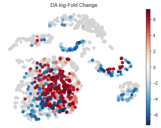
- Milo.plot_nhood_graph(mdata, *, padj_threshold=0.1, min_logFC=0, min_size=10, plot_edges=False, title='DA log-Fold Change', color_map=None, palette=None, ax=None, return_fig=False, alpha=None, **kwargs)[source]#
Visualize DA results on abstracted graph (wrapper around sc.pl.embedding).
- Parameters:
mdata (
MuData) – MuData objectpadj_threshold (
float, default:0.1) – Significance threshold. (default: 0.1)min_logFC (
float, default:0) – Minimum absolute log-Fold Change to show results. If is 0, show all significant neighbourhoods.min_size (
int, default:10) – Minimum size of nodes in visualization. (default: 10)plot_edges (
bool, default:False) – If edges for neighbourhood overlaps whould be plotted.title (
str, default:'DA log-Fold Change') – Plot title.alpha (
float|None, default:None) – Deprecated and will be removed in a future release. Use padj_threshold.return_fig (
bool, default:False) – if True, returns figure of the plot, that can be used for saving.**kwargs – Additional arguments to scanpy.pl.embedding.
- Return type:
Examples
>>> import pertpy as pt
>>> import scanpy as sc
>>> adata = pt.dt.bhattacherjee()
>>> milo = pt.tl.Milo()
>>> mdata = milo.load(adata)
>>> sc.pp.neighbors(mdata["rna"])
>>> sc.tl.umap(mdata["rna"])
>>> milo.make_nhoods(mdata["rna"])
>>> mdata = milo.count_nhoods(mdata, sample_col="orig.ident")
>>> milo.da_nhoods(mdata,
>>>            design='~label',
>>>            model_contrasts='labelwithdraw_15d_Cocaine-labelwithdraw_48h_Cocaine')
>>> milo.build_nhood_graph(mdata)
>>> milo.plot_nhood_graph(mdata)
- Preview: