pertpy.tools.Sccoda#
- class Sccoda(*args, **kwargs)[source]#
Statistical model for single-cell differential composition analysis with specification of a reference cell type.
For further information, see scCODA is a Bayesian model for compositional single-cell data analysis (Büttner, Ostner et al., NatComms, 2021)
Methods table#
|
Decides which effects of the scCODA model are credible based on an adjustable inclusion probability threshold. |
|
Get effect dataframe as printed in the extended summary. |
|
Get intercept dataframe as printed in the extended summary. |
|
Get node effect dataframe as printed in the extended summary of a tascCODA model. |
|
Prepare a MuData object for subsequent processing. |
|
Creates arviz object from model results for MCMC diagnosis. |
|
Implements scCODA model in numpyro. |
|
Grouped boxplot visualization. |
|
Plot a tree with colored circles on the nodes indicating significant effects with bar plots which indicate leave-level significant effects. |
|
Plot a tree using input ete4 tree object. |
|
Barplot visualization for effects. |
|
Plot a UMAP visualization colored by effect strength. |
|
Plots total variance of relative abundance versus minimum relative abundance of all cell types for determination of a reference cell type. |
|
Plots a stacked barplot for all levels of a covariate or all samples (if feature_name=="samples"). |
|
Handles data preprocessing, covariate matrix creation, reference selection, and zero count replacement for scCODA. |
|
Run standard Hamiltonian Monte Carlo sampling (Neal, 2011) to infer optimal model parameters. |
|
Run No-U-turn sampling (Hoffman and Gelman, 2014), an efficient version of Hamiltonian Monte Carlo sampling to infer optimal model parameters. |
|
Direct posterior probability approach to calculate credible effects while keeping the expected FDR at a certain level. |
|
Sets initial MCMC state values for scCODA model. |
|
Printing method for the summary. |
|
Generates summary dataframes for intercepts, effects and node-level effect (if using tree aggregation). |
Methods#
- Sccoda.credible_effects(data, modality_key='coda', est_fdr=None)[source]#
Decides which effects of the scCODA model are credible based on an adjustable inclusion probability threshold.
Note: Parameter est_fdr has no effect for spike-and-slab LASSO selection method.
- Parameters:
- Return type:
- Returns:
Credible effect decision series which includes boolean values indicate whether effects are credible under inc_prob_threshold.
Examples
>>> import pertpy as pt
>>> haber_cells = pt.dt.haber_2017_regions()
>>> sccoda = pt.tl.Sccoda()
>>> mdata = sccoda.load(haber_cells,
>>>                     type="cell_level",
>>>                     generate_sample_level=True,
>>>                     cell_type_identifier="cell_label",
>>>                     sample_identifier="batch",
>>>                     covariate_obs=["condition"])
>>> mdata = sccoda.prepare(mdata, formula="condition", reference_cell_type="Endocrine")
>>> sccoda.run_nuts(mdata, num_warmup=100, num_samples=1000, rng_key=42)
>>> credible_effects = sccoda.credible_effects(mdata).
- Sccoda.get_effect_df(data, modality_key='coda')#
Get effect dataframe as printed in the extended summary.
- Parameters:
- Return type:
- Returns:
Effect data frame.
Examples
>>> import pertpy as pt
>>> haber_cells = pt.dt.haber_2017_regions()
>>> sccoda = pt.tl.Sccoda()
>>> mdata = sccoda.load(haber_cells, type="cell_level", generate_sample_level=True, cell_type_identifier="cell_label",                 sample_identifier="batch", covariate_obs=["condition"])
>>> mdata = sccoda.prepare(mdata, formula="condition", reference_cell_type="Endocrine")
>>> sccoda.run_nuts(mdata, num_warmup=100, num_samples=1000, rng_key=42)
>>> effects = sccoda.get_effect_df(mdata)
- Sccoda.get_intercept_df(data, modality_key='coda')#
Get intercept dataframe as printed in the extended summary.
- Parameters:
- Return type:
- Returns:
Intercept data frame.
Examples
>>> import pertpy as pt
>>> haber_cells = pt.dt.haber_2017_regions()
>>> sccoda = pt.tl.Sccoda()
>>> mdata = sccoda.load(haber_cells, type="cell_level", generate_sample_level=True, cell_type_identifier="cell_label",                 sample_identifier="batch", covariate_obs=["condition"])
>>> mdata = sccoda.prepare(mdata, formula="condition", reference_cell_type="Endocrine")
>>> sccoda.run_nuts(mdata, num_warmup=100, num_samples=1000, rng_key=42)
>>> intercepts = sccoda.get_intercept_df(mdata)
- Sccoda.get_node_df(data, modality_key='coda')#
Get node effect dataframe as printed in the extended summary of a tascCODA model.
- Parameters:
- Return type:
- Returns:
Node effect data frame.
Examples
>>> import pertpy as pt
>>> adata = pt.dt.tasccoda_example()
>>> tasccoda = pt.tl.Tasccoda()
>>> mdata = tasccoda.load(
>>>     adata, type="sample_level",
>>>     levels_agg=["Major_l1", "Major_l2", "Major_l3", "Major_l4", "Cluster"],
>>>     key_added="lineage", add_level_name=True
>>> )
>>> mdata = tasccoda.prepare(
>>>     mdata, formula="Health", reference_cell_type="automatic", tree_key="lineage", pen_args={"phi" : 0}
>>> )
>>> tasccoda.run_nuts(mdata, num_samples=1000, num_warmup=100, rng_key=42)
>>> node_effects = tasccoda.get_node_df(mdata)
- Sccoda.load(adata, type, generate_sample_level=True, cell_type_identifier=None, sample_identifier=None, covariate_uns=None, covariate_obs=None, covariate_df=None, modality_key_1='rna', modality_key_2='coda')[source]#
Prepare a MuData object for subsequent processing. If type is “cell_level”, then create a compositional analysis dataset from the input adata.
When using
type="cell_level",adataneeds to have a column inadata.obsthat contains the cell type assignment. Further, it must contain one column or a set of columns (e.g. subject id, treatment, disease status) that uniquely identify each (statistical) sample. Further covariates (e.g. subject age) can either be specified via addidional column names inadata.obs, a key inadata.uns, or as a separate DataFrame.- Parameters:
adata (
AnnData) – AnnData object.type (
Literal['cell_level','sample_level']) – Specify the input adata type, which could be either a cell-level AnnData or an aggregated sample-level AnnData.generate_sample_level (
bool, default:True) – Whether to generate an AnnData object on the sample level or create an empty AnnData object.cell_type_identifier (
str, default:None) – If type is “cell_level”, specify column name in adata.obs that specifies the cell types.sample_identifier (
str, default:None) – If type is “cell_level”, specify column name in adata.obs that specifies the sample.covariate_uns (
str|None, default:None) – If type is “cell_level”, specify key for adata.uns, where covariate values are stored.covariate_obs (
list[str] |None, default:None) – If type is “cell_level”, specify list of keys for adata.obs, where covariate values are stored.covariate_df (
DataFrame|None, default:None) – If type is “cell_level”, specify dataFrame with covariates.modality_key_1 (
str, default:'rna') – Key to the cell-level AnnData in the MuData object.modality_key_2 (
str, default:'coda') – Key to the aggregated sample-level AnnData object in the MuData object.
- Return type:
- Returns:
mudata.MuDataobject with cell-level AnnData (mudata[modality_key_1]) and aggregated sample-level AnnData (mudata[modality_key_2]).
Examples
>>> import pertpy as pt
>>> haber_cells = pt.dt.haber_2017_regions()
>>> sccoda = pt.tl.Sccoda()
>>> mdata = sccoda.load(haber_cells,
>>>                     type="cell_level",
>>>                     generate_sample_level=True,
>>>                     cell_type_identifier="cell_label",
>>>                     sample_identifier="batch", covariate_obs=["condition"])
- Sccoda.make_arviz(data, modality_key='coda', rng_key=None, num_prior_samples=500, use_posterior_predictive=True)[source]#
Creates arviz object from model results for MCMC diagnosis.
- Parameters:
modality_key (
str, default:'coda') – If data is a MuData object, specify which modality to use.rng_key (
int|None, default:None) – The rng state used for the prior simulation. If None, a random state will be selected.num_prior_samples (
int, default:500) – Number of prior samples calculated.use_posterior_predictive (
bool, default:True) – If True, the posterior predictive will be calculated.
- Returns:
MCMC information
- Return type:
Examples
>>> import pertpy as pt
>>> haber_cells = pt.dt.haber_2017_regions()
>>> sccoda = pt.tl.Sccoda()
>>> mdata = sccoda.load(haber_cells,
>>>                     type="cell_level",
>>>                     generate_sample_level=True,
>>>                     cell_type_identifier="cell_label",
>>>                     sample_identifier="batch",
>>>                     covariate_obs=["condition"])
>>> mdata = sccoda.prepare(mdata, formula="condition", reference_cell_type="Endocrine")
>>> sccoda.run_nuts(mdata, num_warmup=100, num_samples=1000, rng_key=42)
>>> arviz_data = sccoda.make_arviz(mdata, num_prior_samples=100)
- Sccoda.model(counts, covariates, n_total, ref_index, sample_adata)[source]#
Implements scCODA model in numpyro.
- Parameters:
- Returns:
predictions (see numpyro documentation for details on models)
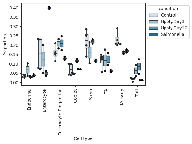
- Sccoda.plot_boxplots(data, feature_name, *, modality_key='coda', y_scale='relative', plot_facets=False, add_dots=False, cell_types=None, args_boxplot=None, args_swarmplot=None, palette='Blues', show_legend=True, level_order=None, figsize=None, dpi=100, layout='long', return_fig=False)#
Grouped boxplot visualization.
The cell counts for each cell type are shown as a group of boxplots with intra–group separation by a covariate from data.obs.
- Parameters:
feature_name (
str) – The name of the feature in data.obs to plotmodality_key (
str, default:'coda') – If data is a MuData object, specify which modality to use.y_scale (
Literal['relative','log','log10','count'], default:'relative') – Transformation to of cell counts. Options: “relative” - Relative abundance, “log” - log(count), “log10” - log10(count), “count” - absolute abundance (cell counts).plot_facets (
bool, default:False) – If False, plot cell types on the x-axis. If True, plot as facets.add_dots (
bool, default:False) – If True, overlay a scatterplot with one dot for each data point.cell_types (
list|None, default:None) – Subset of cell types that should be plotted.args_boxplot (
dict|None, default:None) – Arguments passed to sns.boxplot.args_swarmplot (
dict|None, default:None) – Arguments passed to sns.swarmplot.figsize (
tuple[float,float] |None, default:None) – Figure size.palette (
str|Colormap|None, default:'Blues') – The seaborn color map (name) for the barplot.show_legend (
bool|None, default:True) – If True, adds a legend.level_order (
list[str], default:None) – Custom ordering of bars on the x-axis.layout (
Literal['long','wide'], default:'long') – Controls subplot layout when plot_facets=True. “long”: uses floor(sqrt(K)) resulting in taller layout. “wide”: uses ceil(sqrt(K)) resulting in wider layout.return_fig (
bool, default:False) – if True, returns figure of the plot, that can be used for saving.
- Return type:
- Returns:
If return_fig is True, returns the figure, otherwise None.
Examples
>>> import pertpy as pt
>>> haber_cells = pt.dt.haber_2017_regions()
>>> sccoda = pt.tl.Sccoda()
>>> mdata = sccoda.load(haber_cells, type="cell_level", generate_sample_level=True, cell_type_identifier="cell_label",                 sample_identifier="batch", covariate_obs=["condition"])
>>> sccoda.plot_boxplots(mdata, feature_name="condition", add_dots=True)
- Preview:
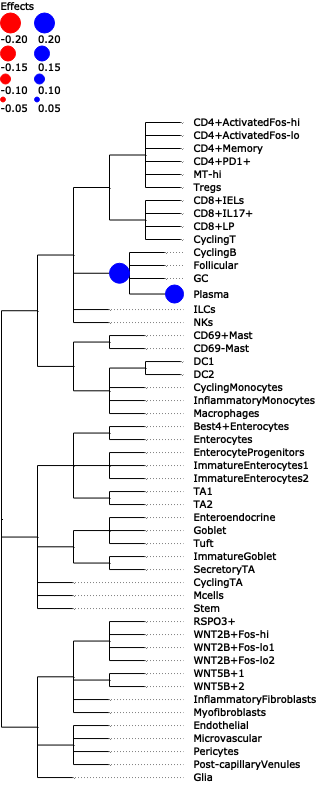
- Sccoda.plot_draw_effects(data, covariate, *, modality_key='coda', tree='tree', show_legend=None, show_leaf_effects=False, tight_text=False, show_scale=False, units='px', figsize=(None, None), dpi=100, save=False, return_fig=False)#
Plot a tree with colored circles on the nodes indicating significant effects with bar plots which indicate leave-level significant effects.
- Parameters:
data (AnnData | MuData) – AnnData object or MuData object.
covariate (str) – The covariate, whose effects should be plotted.
modality_key (str, default:
'coda') – If data is a MuData object, specify which modality to use.tree (str, default:
'tree') – A ete4 tree object or a str to indicate the tree stored in .uns.show_legend (bool | None, default:
None) – If show legend of nodes significant effects or not. Defaults to False if show_leaf_effects is True.show_leaf_effects (bool | None, default:
False) – If True, plot bar plots which indicate leave-level significant effects.tight_text (bool | None, default:
False) – When False, boundaries of the text are approximated according to general font metrics, producing slightly worse aligned text faces but improving the performance of tree visualization in scenes with a lot of text faces.show_scale (bool | None, default:
False) – Include the scale legend in the tree image or not.units (Literal[‘px’, ‘mm’, ‘in’] | None, default:
'px') – Unit of image sizes. “px”: pixels, “mm”: millimeters, “in”: inches.figsize (tuple[float, float] | None, default:
(None, None)) – Figure size.dpi (int | None, default:
100) – Dots per inches.save (str | bool, default:
False) – Save the tree plot to a file. You can specify the file name here.return_fig (bool, default:
False) – if True, returns figure of the plot, that can be used for saving.
- Return type:
Tree | None
- Returns:
Depending on save, returns
ete4.core.tree.Treeandete4.treeview.TreeStyle(save = ‘output.png’) or plot the tree inline (save = False).
Examples
>>> import pertpy as pt
>>> adata = pt.dt.tasccoda_example()
>>> tasccoda = pt.tl.Tasccoda()
>>> mdata = tasccoda.load(
>>>     adata, type="sample_level",
>>>     levels_agg=["Major_l1", "Major_l2", "Major_l3", "Major_l4", "Cluster"],
>>>     key_added="lineage", add_level_name=True
>>> )
>>> mdata = tasccoda.prepare(
>>>     mdata, formula="Health", reference_cell_type="automatic", tree_key="lineage", pen_args=dict(phi=0)
>>> )
>>> tasccoda.run_nuts(mdata, num_samples=1000, num_warmup=100, rng_key=42)
>>> tasccoda.plot_draw_effects(mdata, covariate="Health[T.Inflamed]", tree="lineage")
- Preview:
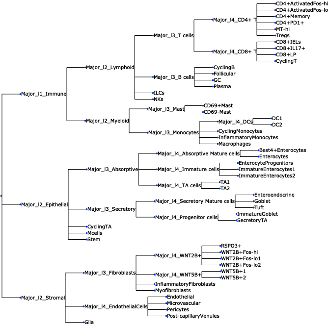
- Sccoda.plot_draw_tree(data, *, modality_key='coda', tree='tree', tight_text=False, show_scale=False, units='px', figsize=(None, None), dpi=100, save=False, return_fig=False)#
Plot a tree using input ete4 tree object.
- Parameters:
data (AnnData | MuData) – AnnData object or MuData object.
modality_key (str, default:
'coda') – If data is a MuData object, specify which modality to use.tree (str, default:
'tree') – A ete4 tree object or a str to indicate the tree stored in .uns.tight_text (bool, default:
False) – When False, boundaries of the text are approximated according to general font metrics, producing slightly worse aligned text faces but improving the performance of tree visualization in scenes with a lot of text faces.show_scale (bool | None, default:
False) – Include the scale legend in the tree image or not.units (Literal[‘px’, ‘mm’, ‘in’] | None, default:
'px') – Unit of image sizes. “px”: pixels, “mm”: millimeters, “in”: inches.figsize (tuple[float, float] | None, default:
(None, None)) – Figure size.dpi (int | None, default:
100) – Dots per inches.save (str | bool, default:
False) – Save the tree plot to a file. You can specify the file name here.return_fig (bool, default:
False) – if True, returns figure of the plot, that can be used for saving.
- Return type:
Tree | None
- Returns:
Depending on save, returns
ete4.core.tree.Treeandete4.treeview.TreeStyle(save = ‘output.png’) or plot the tree inline (save = False)
Examples
>>> import pertpy as pt
>>> adata = pt.dt.tasccoda_example()
>>> tasccoda = pt.tl.Tasccoda()
>>> mdata = tasccoda.load(
>>>     adata, type="sample_level",
>>>     levels_agg=["Major_l1", "Major_l2", "Major_l3", "Major_l4", "Cluster"],
>>>     key_added="lineage", add_level_name=True
>>> )
>>> mdata = tasccoda.prepare(
>>>     mdata, formula="Health", reference_cell_type="automatic", tree_key="lineage", pen_args=dict(phi=0)
>>> )
>>> tasccoda.run_nuts(mdata, num_samples=1000, num_warmup=100, rng_key=42)
>>> tasccoda.plot_draw_tree(mdata, tree="lineage")
- Preview:
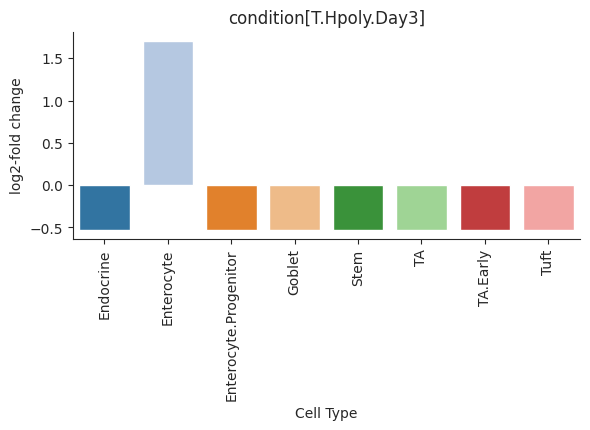
- Sccoda.plot_effects_barplot(data, *, modality_key='coda', covariates=None, parameter='log2-fold change', plot_facets=True, plot_zero_covariate=True, plot_zero_cell_type=False, palette=<matplotlib.colors.ListedColormap object>, level_order=None, args_barplot=None, figsize=None, dpi=100, return_fig=False)#
Barplot visualization for effects.
The effect results for each covariate are shown as a group of barplots, with intra–group separation by cell types. The covariates groups can either be ordered along the x-axis of a single plot (plot_facets=False) or as plot facets (plot_facets=True).
- Parameters:
modality_key (
str, default:'coda') – If data is a MuData object, specify which modality to use.covariates (
str|list|None, default:None) – The name of the covariates in data.obs to plot.parameter (
Literal['log2-fold change','Final Parameter','Expected Sample'], default:'log2-fold change') – The parameter in effect summary to plot.plot_facets (
bool, default:True) – If False, plot cell types on the x-axis. If True, plot as facets.plot_zero_covariate (
bool, default:True) – If True, plot covariate that have all zero effects. If False, do not plot.plot_zero_cell_type (
bool, default:False) – If True, plot cell type that have zero effect. If False, do not plot.figsize (
tuple[float,float] |None, default:None) – Figure size.palette (
str|Colormap|None, default:<matplotlib.colors.ListedColormap object at 0x76f6c91a3050>) – The seaborn color map (name) for the barplot.level_order (
list[str], default:None) – Custom ordering of bars on the x-axis.args_barplot (
dict|None, default:None) – Arguments passed to sns.barplot.return_fig (
bool, default:False) – if True, returns figure of the plot, that can be used for saving.
- Return type:
- Returns:
If return_fig is True, returns the figure, otherwise None.
Examples
>>> import pertpy as pt
>>> haber_cells = pt.dt.haber_2017_regions()
>>> sccoda = pt.tl.Sccoda()
>>> mdata = sccoda.load(haber_cells, type="cell_level", generate_sample_level=True, cell_type_identifier="cell_label",                 sample_identifier="batch", covariate_obs=["condition"])
>>> mdata = sccoda.prepare(mdata, formula="condition", reference_cell_type="Endocrine")
>>> sccoda.run_nuts(mdata, num_warmup=100, num_samples=1000, rng_key=42)
>>> sccoda.plot_effects_barplot(mdata)
- Preview:
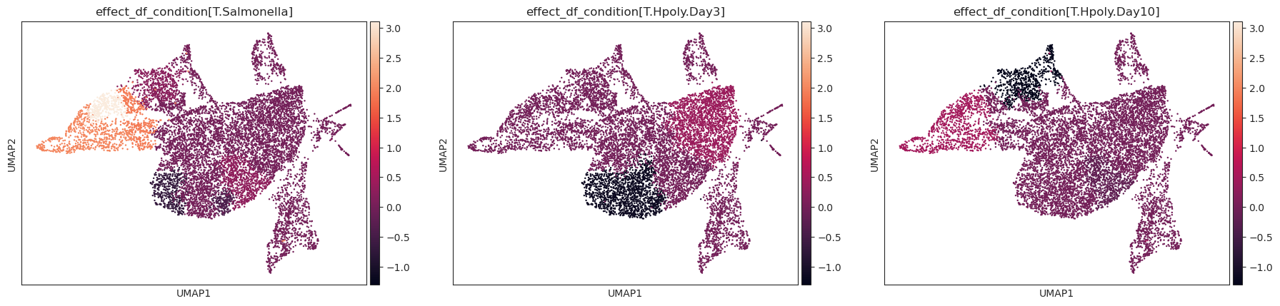
- Sccoda.plot_effects_umap(mdata, effect_name, cluster_key, *, modality_key_1='rna', modality_key_2='coda', color_map=None, palette=None, ax=None, return_fig=False, **kwargs)#
Plot a UMAP visualization colored by effect strength.
Effect results in .varm of aggregated sample-level AnnData (default is data[‘coda’]) are assigned to cell-level AnnData (default is data[‘rna’]) depending on the cluster they were assigned to.
- Parameters:
mdata (
MuData) – MuData object.effect_name (
str|list|None) – The name of the effect results in .varm of aggregated sample-level AnnData to plotcluster_key (
str) – The cluster information in .obs of cell-level AnnData (default is data[‘rna’]). To assign cell types’ effects to original cells.modality_key_1 (
str, default:'rna') – Key to the cell-level AnnData in the MuData object.modality_key_2 (
str, default:'coda') – Key to the aggregated sample-level AnnData object in the MuData object.color_map (
Colormap|str|None, default:None) – The color map to use for plotting.palette (
str|Sequence[str] |Colormap|None, default:None) – The color palette (name) to use for plotting.ax (
Axes, default:None) – A matplotlib axes object. Only works if plotting a single component.return_fig (
bool, default:False) – if True, returns figure of the plot, that can be used for saving.**kwargs – All other keyword arguments are passed to scanpy.plot.umap()
- Return type:
- Returns:
If return_fig is True, returns the figure, otherwise None.
Examples
>>> import pertpy as pt
>>> import scanpy as sc
>>> import schist
>>> adata = pt.dt.haber_2017_regions()
>>> sc.pp.neighbors(adata)
>>> schist.inference.nested_model(adata, n_init=100, random_seed=5678)
>>> tasccoda_model = pt.tl.Tasccoda()
>>> tasccoda_data = tasccoda_model.load(adata, type="cell_level",
>>>                 cell_type_identifier="nsbm_level_1",
>>>                 sample_identifier="batch", covariate_obs=["condition"],
>>>                 levels_orig=["nsbm_level_4", "nsbm_level_3", "nsbm_level_2", "nsbm_level_1"],
>>>                 add_level_name=True)
>>> tasccoda_model.prepare(
>>>     tasccoda_data,
>>>     modality_key="coda",
>>>     reference_cell_type="18",
>>>     formula="condition",
>>>     pen_args=dict(phi=0, lambda_1=3.5),
>>>     tree_key="tree"
>>> )
>>> tasccoda_model.run_nuts(
...     tasccoda_data, modality_key="coda", rng_key=1234, num_samples=10000, num_warmup=1000
... )
>>> sc.tl.umap(tasccoda_data["rna"])
>>> tasccoda_model.plot_effects_umap(tasccoda_data,
>>>                         effect_name=["effect_df_condition[T.Salmonella]",
>>>                                      "effect_df_condition[T.Hpoly.Day3]",
>>>                                      "effect_df_condition[T.Hpoly.Day10]"],
>>>                                       cluster_key="nsbm_level_1",
>>>                         )
- Preview:
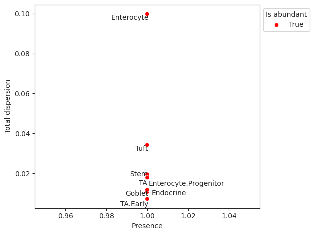
- Sccoda.plot_rel_abundance_dispersion_plot(data, *, modality_key='coda', abundant_threshold=0.9, default_color='Grey', abundant_color='Red', label_cell_types=True, figsize=None, dpi=100, ax=None, return_fig=False)#
Plots total variance of relative abundance versus minimum relative abundance of all cell types for determination of a reference cell type.
If the count of the cell type is larger than 0 in more than abundant_threshold percent of all samples, the cell type will be marked in a different color.
- Parameters:
modality_key (
str, default:'coda') – If data is a MuData object, specify which modality to use.abundant_threshold (
float|None, default:0.9) – Presence threshold for abundant cell types.default_color (
str|None, default:'Grey') – Bar color for all non-minimal cell types.abundant_color (
str|None, default:'Red') – Bar color for cell types with abundant percentage larger than abundant_threshold.label_cell_types (
bool, default:True) – Label dots with cell type names.figsize (
tuple[float,float] |None, default:None) – Figure size.ax (
Axes|None, default:None) – A matplotlib axes object. Only works if plotting a single component.return_fig (
bool, default:False) – if True, returns figure of the plot, that can be used for saving.
- Return type:
- Returns:
If return_fig is True, returns the figure, otherwise None.
Examples
>>> import pertpy as pt
>>> haber_cells = pt.dt.haber_2017_regions()
>>> sccoda = pt.tl.Sccoda()
>>> mdata = sccoda.load(haber_cells, type="cell_level", generate_sample_level=True, cell_type_identifier="cell_label",                 sample_identifier="batch", covariate_obs=["condition"])
>>> mdata = sccoda.prepare(mdata, formula="condition", reference_cell_type="Endocrine")
>>> sccoda.run_nuts(mdata, num_warmup=100, num_samples=1000, rng_key=42)
>>> sccoda.plot_rel_abundance_dispersion_plot(mdata)
- Preview:
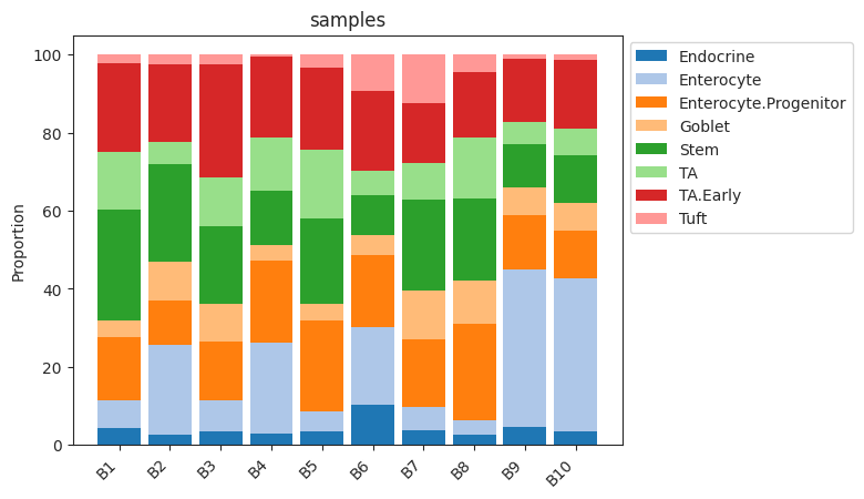
- Sccoda.plot_stacked_barplot(data, feature_name, *, modality_key='coda', palette=<matplotlib.colors.ListedColormap object>, show_legend=True, level_order=None, figsize=None, dpi=100, return_fig=False)#
Plots a stacked barplot for all levels of a covariate or all samples (if feature_name==”samples”).
- Parameters:
feature_name (
str) – The name of the covariate to plot. If feature_name==”samples”, one bar for every sample will be plottedmodality_key (
str, default:'coda') – If data is a MuData object, specify which modality to use.figsize (
tuple[float,float] |None, default:None) – Figure size.palette (
str|Colormap|None, default:<matplotlib.colors.ListedColormap object at 0x76f6c91a3050>) – The matplotlib color map (name) for the barplot.show_legend (
bool|None, default:True) – If True, adds a legend.level_order (
list[str], default:None) – Custom ordering of bars on the x-axis.return_fig (
bool, default:False) – if True, returns figure of the plot, that can be used for saving.
- Return type:
- Returns:
If return_fig is True, returns the Figure, otherwise None.
Examples
>>> import pertpy as pt
>>> haber_cells = pt.dt.haber_2017_regions()
>>> sccoda = pt.tl.Sccoda()
>>> mdata = sccoda.load(haber_cells, type="cell_level", generate_sample_level=True, cell_type_identifier="cell_label",                 sample_identifier="batch", covariate_obs=["condition"])
>>> sccoda.plot_stacked_barplot(mdata, feature_name="samples")
- Preview:
- Sccoda.prepare(data, formula, reference_cell_type='automatic', automatic_reference_absence_threshold=0.05, modality_key='coda')[source]#
Handles data preprocessing, covariate matrix creation, reference selection, and zero count replacement for scCODA.
- Parameters:
data (
AnnData|MuData) – Anndata object with cell counts as sample_adata.X and covariates saved in sample_adata.obs.formula (
str) – R-style formula for building the covariate matrix. Categorical covariates are handled automatically, with the covariate value of the first sample being used as the reference category. To set a different level as the base category for a categorical covariate, use “C(<CovariateName>, Treatment(‘<ReferenceLevelName>’))”reference_cell_type (
str, default:'automatic') – Column name that sets the reference cell type. Reference the name of a column. If “automatic”, the cell type with the lowest dispersion in relative abundance that is present in at least 90% of samlpes will be chosen.automatic_reference_absence_threshold (
float, default:0.05) – If using reference_cell_type = “automatic”, determine the maximum fraction of zero entries for a cell type to be considered as a possible reference cell type.modality_key (
str, default:'coda') – If data is a MuData object, specify key to the aggregated sample-level AnnData object in the MuData object.
- Return type:
- Returns:
Return an AnnData (if input data is an AnnData object) or return a MuData (if input data is a MuData object)
Specifically, parameters have been set:
adata.uns[“param_names”] or data[modality_key].uns[“param_names”]: List with the names of all tracked latent model parameters (through npy.sample or npy.deterministic)
adata.uns[“scCODA_params”][“model_type”] or data[modality_key].uns[“scCODA_params”][“model_type”]: String indicating the model type (“classic”)
adata.uns[“scCODA_params”][“select_type”] or data[modality_key].uns[“scCODA_params”][“select_type”]: String indicating the type of spike_and_slab selection (“spikeslab”)
Examples
>>> import pertpy as pt
>>> haber_cells = pt.dt.haber_2017_regions()
>>> sccoda = pt.tl.Sccoda()
>>> mdata = sccoda.load(haber_cells,
>>>                     type="cell_level",
>>>                     generate_sample_level=True,
>>>                     cell_type_identifier="cell_label",
>>>                     sample_identifier="batch",
>>>                     covariate_obs=["condition"])
>>> mdata = sccoda.prepare(mdata, formula="condition", reference_cell_type="Endocrine")
- Sccoda.run_hmc(data, modality_key='coda', num_samples=20000, num_warmup=5000, rng_key=None, copy=False, *args, **kwargs)#
Run standard Hamiltonian Monte Carlo sampling (Neal, 2011) to infer optimal model parameters.
- Parameters:
modality_key (
str, default:'coda') – If data is a MuData object, specify which modality to use.num_samples (
int, default:20000) – Number of sampled values after burn-in.num_warmup (
int, default:5000) – Number of burn-in (warmup) samples.rng_key (default:
None) – The rng state used. If None, a random state will be selected.copy (
bool, default:False) – Return a copy instead of writing to adata.*args – Additional args passed to numpyro HMC
**kwargs – Additional kwargs passed to numpyro HMC
Examples
>>> import pertpy as pt
>>> haber_cells = pt.dt.haber_2017_regions()
>>> sccoda = pt.tl.Sccoda()
>>> mdata = sccoda.load(haber_cells, type="cell_level", generate_sample_level=True, cell_type_identifier="cell_label",                 sample_identifier="batch", covariate_obs=["condition"])
>>> mdata = sccoda.prepare(mdata, formula="condition", reference_cell_type="Endocrine")
>>> sccoda.run_hmc(mdata, num_warmup=100, num_samples=1000)
- Sccoda.run_nuts(data, modality_key='coda', num_samples=10000, num_warmup=1000, rng_key=0, copy=False, *args, **kwargs)[source]#
Run No-U-turn sampling (Hoffman and Gelman, 2014), an efficient version of Hamiltonian Monte Carlo sampling to infer optimal model parameters.
- Parameters:
modality_key (
str, default:'coda') – If data is a MuData object, specify which modality to use.num_samples (
int, default:10000) – Number of sampled values after burn-in.num_warmup (
int, default:1000) – Number of burn-in (warmup) samples.rng_key (
int, default:0) – The rng state used.copy (
bool, default:False) – Return a copy instead of writing to adata.*args – Additional args passed to numpyro NUTS
**kwargs – Additional kwargs passed to numpyro NUTS
- Returns:
Calls self.__run_mcmc
Examples
>>> import pertpy as pt
>>> haber_cells = pt.dt.haber_2017_regions()
>>> sccoda = pt.tl.Sccoda()
>>> mdata = sccoda.load(haber_cells,
>>>                     type="cell_level",
>>>                     generate_sample_level=True,
>>>                     cell_type_identifier="cell_label",
>>>                     sample_identifier="batch",
>>>                     covariate_obs=["condition"])
>>> mdata = sccoda.prepare(mdata, formula="condition", reference_cell_type="Endocrine")
>>> sccoda.run_nuts(mdata, num_warmup=100, num_samples=1000, rng_key=42).
- Sccoda.set_fdr(data, est_fdr, modality_key='coda', *args, **kwargs)[source]#
Direct posterior probability approach to calculate credible effects while keeping the expected FDR at a certain level.
Note: Does not work for spike-and-slab LASSO selection method.
- Parameters:
- Returns:
Adjusts intercept_df and effect_df
Examples
>>> import pertpy as pt
>>> haber_cells = pt.dt.haber_2017_regions()
>>> sccoda = pt.tl.Sccoda()
>>> mdata = sccoda.load(haber_cells,
>>>                     type="cell_level",
>>>                     generate_sample_level=True,
>>>                     cell_type_identifier="cell_label",
>>>                     sample_identifier="batch",
>>>                     covariate_obs=["condition"])
>>> mdata = sccoda.prepare(mdata, formula="condition", reference_cell_type="Endocrine")
>>> sccoda.run_nuts(mdata, num_warmup=100, num_samples=1000, rng_key=42)
>>> sccoda.set_fdr(mdata, est_fdr=0.4).
- Sccoda.set_init_mcmc_states(rng_key, ref_index, sample_adata)[source]#
Sets initial MCMC state values for scCODA model.
- Parameters:
- Return type:
- Returns:
Return AnnData object.
Examples
>>> import pertpy as pt
>>> haber_cells = pt.dt.haber_2017_regions()
>>> sccoda = pt.tl.Sccoda()
>>> mdata = sccoda.load(haber_cells,
>>>                     type="cell_level",
>>>                     generate_sample_level=True,
>>>                     cell_type_identifier="cell_label",
>>>                     sample_identifier="batch",
>>>                     covariate_obs=["condition"])
>>> mdata = sccoda.prepare(mdata, formula="condition", reference_cell_type="Endocrine")
>>> adata = sccoda.set_init_mcmc_states(rng_key=42, ref_index=0, sample_adata=mdata["coda"])
- Sccoda.summary(data, extended=False, modality_key='coda', *args, **kwargs)[source]#
Printing method for the summary.
- Parameters:
Examples
>>> import pertpy as pt
>>> haber_cells = pt.dt.haber_2017_regions()
>>> sccoda = pt.tl.Sccoda()
>>> mdata = sccoda.load(haber_cells, type="cell_level", generate_sample_level=True, cell_type_identifier="cell_label",                 sample_identifier="batch", covariate_obs=["condition"])
>>> mdata = sccoda.prepare(mdata, formula="condition", reference_cell_type="Endocrine")
>>> sccoda.run_nuts(mdata, num_warmup=100, num_samples=1000, rng_key=42)
>>> sccoda.summary(mdata)
Examples
>>> import pertpy as pt
>>> haber_cells = pt.dt.haber_2017_regions()
>>> sccoda = pt.tl.Sccoda()
>>> mdata = sccoda.load(haber_cells,
>>>                     type="cell_level",
>>>                     generate_sample_level=True,
>>>                     cell_type_identifier="cell_label",
>>>                     sample_identifier="batch",
>>>                     covariate_obs=["condition"])
>>> mdata = sccoda.prepare(mdata, formula="condition", reference_cell_type="Endocrine")
>>> sccoda.run_nuts(mdata, num_warmup=100, num_samples=1000, rng_key=42)
>>> sccoda.summary(mdata).
- Sccoda.summary_prepare(sample_adata, est_fdr=0.05, *args, **kwargs)#
Generates summary dataframes for intercepts, effects and node-level effect (if using tree aggregation).
This function builds on and supports all functionalities from
az.summary.- Parameters:
- Returns:
class:pandas.DataFrame, :class:pandas.DataFrame] or Tuple[:class:pandas.DataFrame, :class:pandas.DataFrame, :class:pandas.DataFrame]: Intercept, effect and node-level DataFrames
- intercept_df
Summary of intercept parameters. Contains one row per cell type.
Final Parameter: Final intercept model parameter
HDI X%: Upper and lower boundaries of confidence interval (width specified via hdi_prob=)
SD: Standard deviation of MCMC samples
Expected sample: Expected cell counts for a sample with no present covariates. See the tutorial for more explanation
- effect_df
Summary of effect (slope) parameters. Contains one row per covariate/cell type combination.
Final Parameter: Final effect model parameter. If this parameter is 0, the effect is not significant, else it is.
HDI X%: Upper and lower boundaries of confidence interval (width specified via hdi_prob=)
SD: Standard deviation of MCMC samples
Expected sample: Expected cell counts for a sample with only the current covariate set to 1. See the tutorial for more explanation
log2-fold change: Log2-fold change between expected cell counts with no covariates and with only the current covariate. This is a compositional fold change — expected counts are re-normalized to the same total per sample before the ratio is taken. Because of that re-normalization, the sign of
log2-fold changecan disagree with the sign ofFinal Parameter: a cell type withFinal Parameter = 0can still have a non-zero log2-fold change driven entirely by other cell types’ effects, and a cell type with a small negativeFinal Parametercan have a positive log2-fold change if other cell types are shifting down faster.Inclusion probability: Share of MCMC samples, for which this effect was not set to 0 by the spike-and-slab prior.
- node_df
Summary of effect (slope) parameters on the tree nodes (features or groups of features). Contains one row per covariate/cell type combination.
Final Parameter: Final effect model parameter. If this parameter is 0, the effect is not significant, else it is.
Median: Median of parameter over MCMC chain
HDI X%: Upper and lower boundaries of confidence interval (width specified via hdi_prob=)
SD: Standard deviation of MCMC samples
Delta: Decision boundary value - threshold of practical significance
Is credible: Boolean indicator whether effect is credible
- Return type:
tuple[DataFrame,DataFrame] |tuple[DataFrame,DataFrame,DataFrame]
Examples
>>> import pertpy as pt
>>> haber_cells = pt.dt.haber_2017_regions()
>>> sccoda = pt.tl.Sccoda()
>>> mdata = sccoda.load(haber_cells, type="cell_level", generate_sample_level=True, cell_type_identifier="cell_label",                 sample_identifier="batch", covariate_obs=["condition"])
>>> mdata = sccoda.prepare(mdata, formula="condition", reference_cell_type="Endocrine")
>>> sccoda.run_nuts(mdata, num_warmup=100, num_samples=1000, rng_key=42)
>>> intercept_df, effect_df = sccoda.summary_prepare(mdata["coda"])